Lecture 22: Data pipelines

Image credit: Randall Munroe https://xkcd.com/2054/

Matt Graham

Centre for Advanced Research Computing

Anastasis Georgoulas

Introduction

We are going to step back a bit from the details of fitting specific classes of machine learning models as covered in the earlier lectures, and instead look at some of the wider issues involved in managing the data and model outputs we accumulate during data science projects. This comes under the umbrella of what is sometimes termed machine learning operations or MLOps for short.

The sorts of questions we will consider include

• How to store and access datasets hosted remotely.
• How to manage the multiple versions of datasets and models we produce during a typical project.
• And how to ensure our analyses are reproducible.

Importantly we will also cover some useful tools that can help streamlines our workflows and ensure they can be reproduced by others.

We will begin by considering how we structure our overall workflows, including not just the model fitting process but the stages that feed in and out of this.

Applying machine learning algorithms and approaches to real-world data involves a number of practical challenges. In this series of lectures, we will look at tools and ways of working that address questions like:

• How can I store and access large amounts of data remotely?
• How can I keep track of different versions of datasets?
• How can I share my results and make my analyses reproducible by others?

We’ll begin with the broader picture of how we handle data.

Learning outcomes

• Recognize that model training is just one part of machine learning workflows.
• Describe key typical stages of data pipelines.
• Identify the benefits of defining data pipelines programmatically.
• Explain the importance of the FAIR principles for data management.

Data preparation

Typically before we train any machine learning model there will steps we need to go through to get the data into the format required to fit the model, and potentially also to get hold of the data in the first place.

For example,

• we may need to access the data from some remote repository,
• the data may need cleaning or other preprocessing,
• we may need to transform the raw data to generate the features required for training the model,
• we may need to serve the data in a particular way for it to be consumable by the model,
• once the model is fitted we may wish to share it with others.

Typically the data of interest will not be directly useable.

Before we can train any model, we first need to make sure that the data is available and properly formatted.

This can involve a number of steps:

• Accessing the data.
• Cleaning and other preprocessing.
• Transforming and generating features.
• Making the data available to the model.

The data is then ready to be used in our algorithm of choice.

Pipelines

The overall sequences of steps involved in such a typical machine learning workflow is sometimes called a data pipeline, with related terms such as extract-transform-load or ETL also being used.

We can visualise this as a data flow graph as shown here. To ensure reproducibility ideally all stages in the pipeline should be defined programmatically through code rather than requiring manual actions. We’ll now go through and explain what might be involved in each of these stages, and use running example of analysing historical climate records data to illustrate an concrete example of a data pipeline.

This sequence of steps is sometimes called a data pipeline.

Another related term used to describe similar workflows is ETL: Extract-Transform-Load.

When possible, it is useful to perform these steps programmatically (through code) rather than manually.

Accessing data

Commonly the first step in any data science project will be to get hold of the data we will be analysing, unless we happen to have collected it ourselves. This typically happens in a variety of different ways, for example:

• we get sent a data file by a colleague,
• we pull the data from some web service,
• we might run a scraper to extract data from a website,
• or we might execute a query to a database we have access to.

If we haven’t collected the data ourselves, we will first need to access it. This can be done in a number of ways. For example:

• A colleague gives us a file.
• We connect to a web service that produces the data.
• We “scrape” a web page or other source to extract the data.
• We query a database for the particular data we want.

Accessing data

It will often be the case that we in fact have to combine data from multiple different sources. We will discuss some of the intricacies of querying data from a database in a later lecture.

A unifying aspect of most of these examples is that the data is hosted remotely on a different computer. How specifically we access it will depend on the details of the remote host, the format of the data and its sizes, however importantly the steps to access the data can often be defined programatically.

Sometimes we will need to combine more than one source to get the full set of data that we require.

We will talk more about databases in a subsequent lecture.

A common element in the above examples is that the data can exist in some remote location.

How we get it on our own computer will depend on the source, format and size of the data. However, this can often be done programmatically.

Example: Downloading climate data

To give an example of how we might access data programmatically, we will consider how to download a set of historical global climate records from an open dataset hosted on Simple Storage Service (S3) that is part of the Amazon Web Services (AWS) cloud offering.

In this example we will use the Python standard library module urllib.request which allows programmatically accessing data hosted on the web via hypertext transfer protocol (HTTP). In more complex cases, for example where access to an S3 bucket requires authentication, the Python package boto3 is a dedicated Python package for interacting with AWS services programmatically.

Simple Storage Service (S3) is a storage service offered by Amazon Web Services (AWS).

Users can upload datasets which can be accessed by others.

As a running example we will look at an open dataset of historical global climate records.

Example: Downloading climate data

The particular data we will be using are the climate records from the year 1800, which are held in an S3 bucket noaa-ghcn-pds in tabular format as a comma separated variable (CSV) file, which has been compressed using gzip. Python has a built-in module gzip which can be used to uncompress the file and we will use Pandas to read in the data to a dataframe.

We download climate records for the year 1800 from a AWS S3 bucket noaa-ghcn-pds. The data is stored as a comma separated variable (CSV) file compressed using gzip.

import urllib.request
import gzip
import pandas

data_url = "https://noaa-ghcn-pds.s3.amazonaws.com/csv.gz/1800.csv.gz"
with urllib.request.urlopen(data_url) as response:
    with gzip.open(response, "rb") as f:
        input_data = pandas.read_csv(
            f, usecols=range(4), names=["station", "date", "quantity", "value"]
        )
display(input_data.head())

	station	date	quantity	value
0	EZE00100082	18000101	TMAX	-86
1	EZE00100082	18000101	TMIN	-135
2	GM000010962	18000101	PRCP	0
3	ITE00100554	18000101	TMAX	-75
4	ITE00100554	18000101	TMIN	-148

Preprocessing

Typically getting access to the data we need is only the first step, with often the raw data needing to be preprocessed before use. This might be for example because,

• there are errors in the data,
• the dimensionality of each data point or number of data points is too large for us to be able to use directly,
• the data contains irrelevant information for our analysis,
• the variables in the raw data do not directly correspond to quantities of interest which need to be derived from the raw data,
• there may be outliers or imbalances in the dataset that might affect the fitting of some models.

Getting hold of the data you want to work with is only the first step. Sometimes this raw or preliminary data has to be changed. There are many reasons why:

• Data may contain errors.
• Dimensionality or size of dataset is too high.
• We want to focus only on a subset of interest.
• Raw data does not directly contain variables of interest.
• Some algorithms are negatively impacted by e.g. imbalances in class frequencies or extreme values.

Preprocessing

The sorts of preprocessing steps we might perform to address these issues include,

• removing problematic values from the data,
• filtering the data to a smaller subset or augmenting it by repeating samples.

This process is sometimes referred to as data cleaning, and is a vital and often overlooked stage in data pipelines. While such cleaning steps can be performed manually, tools such as OpenRefine have been developed to help automate the process.

Preprocessing steps can include:

• Replacing values that are incorrect or cause problems.
• Filtering, subsampling (discarding samples) or supersampling (repeating samples).
• Removing outliers.

Aspects of this are often referred to as cleaning the data.

This is an important and often undervalued pipeline step.

These transformations can be performed manually, although tools like OpenRefine can simplify and automate the process.

Example: filtering climate records

Returning to our running climate data example, at the end of the previous stage of our pipeline we had the data loaded into a dataframe input_data containing climate records for the year 1800 for multiple different land-observation stations. We will assume we are interested in fitting a model to daily temperature range recorded for a single station. This will mean we will need to preprocess the input data to filter for the records associated with a particular station.

Continuing with the climate data example, the dataframe input_data we loaded contains climate records for multiple different land-observation stations.

We might wish to fit a model to the daily extreme temperature records for a single station.

We therefore need to filter the input data to leave only the temperature measurements associated with this station.

Example: filtering climate records

Specifically here we will look for the records recorded at a station in Milan, Italy and use the Pandas DataFrame.query method to perform the filtering.

Using station ITE00100554 (in Milan, Italy) as an example we can achieve this for example using the DataFrame.query method in Pandas.

preprocessed_data = input_data.query(
    'station == "ITE00100554" and quantity in ["TMIN", "TMAX"]'
)
display(preprocessed_data.head())

	station	date	quantity	value
3	ITE00100554	18000101	TMAX	-75
4	ITE00100554	18000101	TMIN	-148
8	ITE00100554	18000102	TMAX	-60
9	ITE00100554	18000102	TMIN	-125
13	ITE00100554	18000103	TMAX	-23

Transforming

Once we have performed any necessary cleaning and preprocessing of the data, while closer to have data in the form necessary for model fitting, often we will need go through further stages of data processing first. A very common requirement is to generate features suitable for training the model from the variables present in the raw data.

Cleaning brings you one step closer to useable data inputs for your model.

However, your analysis may rely on variables that are not directly present in the original data.

There is therefore a need for feature generation: extracting the variables of interest by combining existing ones.

Example: transforming to temperature range time series

Going back to our running example again, after the preprocessing step we have a dataframe preprocessed_data containing records of all the daily minimum and maximum temperature measurements, in tenths of a degree Celsius, for each day in 1800 for the station of interest in Milan. Our aim is to fit a model to the daily temperature range in degrees Celsius against the date, and so we need to process the dataframe to produce the required variates and covariates for regression.

The preprocessed_data dataframe we computed previously contains rows with individual TMIN and TMAX measurements (daily minimum and maximum temperatures in tenths of a degree Celsius) for each day in 1800.

If we wish to fit a regression model of the daily temperature range in degrees Celsius against the date we need to transform the data in the preprocessed_data dataframe accordingly.

Example: transforming to temperature range time series

pivoted_data = preprocessed_data.pivot(
    index="date", columns="quantity", values="value"
)
pivoted_data.index = pandas.to_datetime(pivoted_data.index, format="%Y%m%d")
display(pivoted_data.head())

quantity	TMAX	TMIN
date
1800-01-01	-75	-148
1800-01-02	-60	-125
1800-01-03	-23	-46
1800-01-04	0	-13
1800-01-05	10	-6

Example: transforming to temperature range time series

transformed_data = pandas.DataFrame(
    {"temperature_range": (pivoted_data.TMAX - pivoted_data.TMIN) / 10}
)
display(transformed_data.head())

	temperature_range
date
1800-01-01	7.3
1800-01-02	6.5
1800-01-03	2.3
1800-01-04	1.3
1800-01-05	1.6

Serving

The code to trained a model will often require data to be provided in a particular format. After we have finished preprocessing the data we therefore still need to ensure the data is served to the model in the correct format for consumption by the model.

The code you have written may expect to read in data in a particular format, such as a CSV file, or a collection of files.

The result of your preprocessing must therefore be made available in the same format.

Serving

The data can be served to a model in a variety of ways - while file based input-output is common, in other cases we might for example make the data available via a web service. They key point is the data needs to be in the format required to feed to the model.

Note that the result of this step need not be a file on your computer: you could choose to serve your data through, for example, a web service.

The important thing is that, at the end of this step, the data is ready to be fed into the model, matching what that code expects.

Serving

Libraries such as Pandas provide a variety of functions for reading from and writing to data in a range of commonly used formats - for example JSON or CSV files.

This preparation can often be done through a library. For instance, pandas offers several methods for writing out a data frame to a number of commonly-used formats:

import pandas as pd
df = pd.read_json('my_data.json')
# ...Perform any transformations...
df.to_csv('my_ready_data.csv')

Example: serving for scikit-learn

In previous lectures you have seen that scikit-learn requires that the training data provided to regression models is formatted as a features matrix with rows corresponding to the numeric features of each training data point and a one-dimensional target array containing the target values for each training data point.

As seen in a previous lecture, scikit-learn models expect the training data for regression problems to be formatted as

• a features matrix, with each row corresponding to the (numeric) features for each training datapoint,
• and a target array, a one-dimensional array containing the target values for each training datapoint.

Example: serving for scikit-learn

For our running example we will convert the measurement dates to integer days of the year as the input features, so that they are of a numeric type as required. For the target outputs we will use the temperature ranges.

Here we use the measurement dates converted to integer days of the year as the input features and the temperature ranges as the target values.

import matplotlib.pyplot as plt

X_train = transformed_data.index.day_of_year.array[:, None]
y_train = transformed_data.temperature_range.array
fig, ax = plt.subplots(figsize=(8, 3))
ax.plot(X_train, y_train)
ax.set(xlabel="Day of year", ylabel=r"Daily temperature range / $^\circ C$")
fig.tight_layout()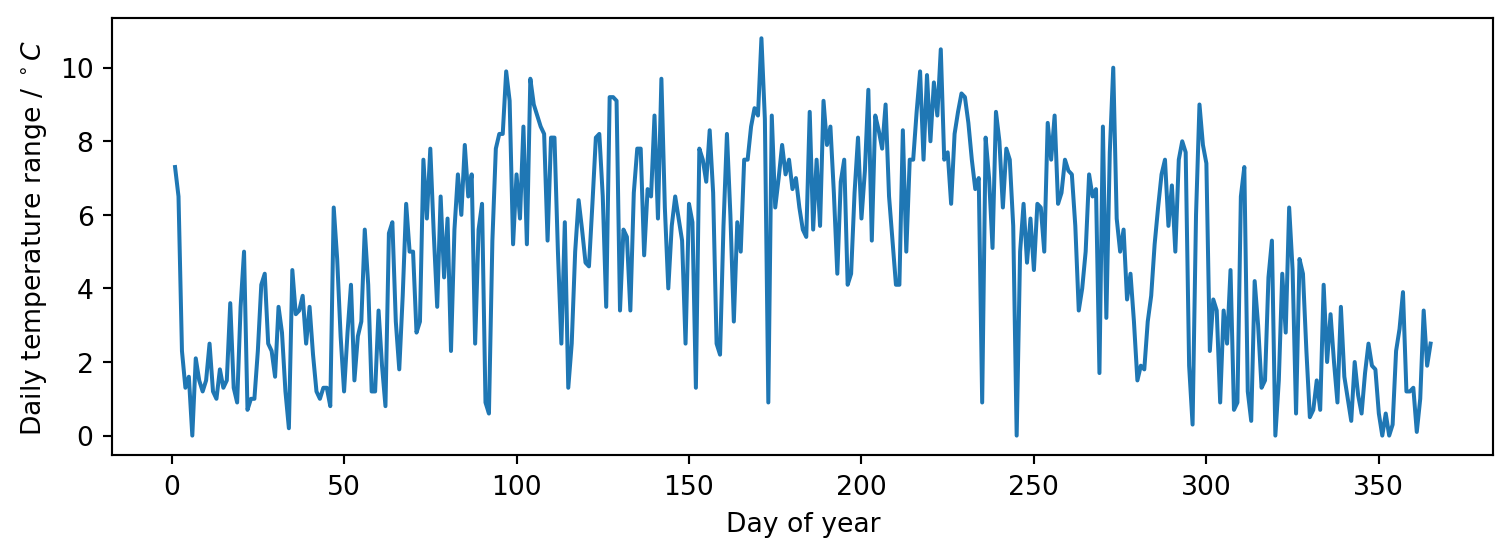

Model fitting

When we finally have the data served in the format required for feeding to the model we are ready to begin training, or potentially prediction using an existing trained model. This could involve any of the different model types and Python packages such as scikit-learn and TensorFlow, that have been covered in the preceding lectures.

As an aside, it is important to note that both scikit-learn and TensorFlow internally make use of the concept of data pipelines when building models.

Once we have data in expected format we can fit a model using any of approaches seen in the previous lectures - for example scikit-learn or TensorFlow.

Note that both scikit-learn and TensorFlow themselves use data pipelines concept as an abstraction when building models - see for example the scikit-learn documentation for the Pipeline class.

Model fitting

Where we consider the dividing line between the model and other data pipeline stages may therefore in practice not always be that clear cut as the model itself may be a composition of multiple components, including steps we might consider as feature extraction or transformations. For example, commonly the earlier layers of deep neural network models are considered as feature extractors feeding into a regressor or classifier in the final layer.

When we refer to ‘a model’ we therefore are often actually referring to something that is itself a composition of multiple components, including steps we might consider as preprocessing or transforming.

The boundaries between the model and other stages in the pipeline we have described in reality may not always be as clear cut as in our simple flowchart.

Example: fitting a periodic spline

Again returning to our running climate data example, we will illustrate fitting the noisy temperature range time series data we previously observed with a spline model in scikit-learn. Splines are a flexible way of describing smooth relationships between variables using piecewise polynomials constrained to ensure smoothness at the join points. They are parametrized by a set of knot points defining how the input space is partitioned, and a positive integer degree specifying the exponent of the highest order polynomial term used.

As we saw when plotting the data, there appears to be an underlying seasonal trend in the time series, and so we will additionally enforce that the model is periodic with period one year. We will use a spline with 7 knots, corresponding to partitioning the input time interval into 6 roughly bimonthly intervals, with this allowing capturing a smooth representation of the overall seasonal trends without overfitting to the noisy daily variation.

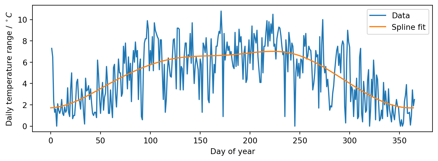
We can fit a spline model using scikit-learn to smoothly interpolate our running example dataset.

As we have time series data of daily temperature ranges for a full year and expect the dominant trends to be seasonal, enforce that the fitted model is periodic.

We fit a cubic spline with seven knots at roughly bimonthly intervals so that we capture a smooth representation of the overall seasonal trends rather than the noisy daily variation.

Example: fitting a periodic spline

import numpy
from sklearn import pipeline, preprocessing, linear_model

model = pipeline.make_pipeline(
    preprocessing.SplineTransformer(
        degree=3,
        knots=numpy.linspace(1, 365, 7)[:, None],
        extrapolation="periodic"
    ),
    linear_model.Ridge()
)
model.fit(X_train, y_train)

Pipeline(steps=[('splinetransformer',
                 SplineTransformer(extrapolation='periodic',
                                   knots=array([[  1.        ],
       [ 61.66666667],
       [122.33333333],
       [183.        ],
       [243.66666667],
       [304.33333333],
       [365.        ]]))),
                ('ridge', Ridge())])

In a Jupyter environment, please rerun this cell to show the HTML representation or trust the notebook.
On GitHub, the HTML representation is unable to render, please try loading this page with nbviewer.org.

Example: fitting a periodic spline

We can visualise the fitted model’s predictions over the input range to check they look reasonable using matplotlib

fig, ax = plt.subplots(figsize=(8, 3))
ax.plot(X_train, y_train, model.predict(X_train))
ax.set(xlabel="Day of year", ylabel=r"Daily temperature range / $^\circ C$")
ax.legend(["Data", "Spline fit"])
fig.tight_layout()

Publishing

Once we have trained our model or used it to produce predictions, our job is still often not yet done. The model itself and the outputs we generate using it can be considered as new data to be shared with others to allow them to reproduce our analyses and reuse the results in their own analysis.

We might therefore wish to host our model or model outputs on a platform that allows others to access them. A simple option would be to simply place the files on cloud storage service such as the Amazon Web Services Simple Storage Service we encountered previously. While a viable route for giving others access to the model files themselves, in general to ensure our data is amenable to reuse by others as possible we need to do some further work.

One particular route that can be worth considering is to use a specialised repositories for hosting research data and other digital assets such as Zenodo or institutional equivalents such as the UCL Research Data Repository. Compared to generic cloud storage services these offer more features for helping to ensure the way we share our data aligns with what are called the FAIR principles of findability, accessibility, interoperability and reusability, that we will cover in more detail shortly.

The lifecycle of data does not have to end when you feed it into a model!

You can even think of the model itself, and any analyses (e.g. predictions) you make based on it, as new data.

These can in turn be made available to support further research or other work.

You may want to consider uploading them to cloud storage (like S3) or a data repository like Zenodo.

Publishing data

A key consideration when releasing and data is the format it will be stored in. Typically it is better to distribute data either in generic widely supported open data formats - for example comma separated variable (CSV) files for tabular data or JavaScript Object Notation (JSON) files for structured data, or in a formats that are standard to a particular field, for example NetCDF files for geoscientific data or DICOM for medical imaging data. Likewise it is best to avoid where possible non-open file formats that require proprietary software to read such as Excel workbooks or MATLAB data files, to ensure the data is as usable by as wide an audience as possible.

A very important point is that as well as publishing the data itself, you should also distribute the data with descriptive metadata which describes for example, the provenance of the data, that is how it was generated and where any data that fed into it came from, and documents what is included within the data and how to interpret it.

When releasing your datasets, it is useful to put them in a standard format (such as CSV or JSON) that will be easy for others to read.

You should also include metadata that explains how the data was generated and what it contains.

FAIR principles

When publishing data or other digital assets, a useful framework to follow are what are called the FAIR principles, which where first defined in a research article in Scientific Data by a consortium of scientists and research organizations in March 2016.

A key consideration underlying the FAIR principles are that the shared data and metadata should be machine actionable - that is able to be used with minimal human intervention. The four principles are defined as

• Findability - the idea that potential users should be able to search for a shared data artefact via some index. This is linked to a requirement that the data is assigned a unique and persistent global identifier so that it can indexed and also refound and referred to later, and that it is described with a rich set of metadata that facilitate searching.
• Accessibility - this refers to the principle that how data can be accessed must be clearly documented, ideally by allowing use of a standardized communication protocol for accessing the data and its attached metatdata via its unique global identifier.
• Interoperability - this encapsulates the need for the shared data artefact to be able to be integrated with other data and software. A key consideration here is the format in which both the data and any attached metadata is distributed.
• Reusability - the overall aim of the FAIR principles are to facilitate reuse of data. This both requires that the data is richly described by metadata that explain its provenance and how it is structured, but also that the terms of reuse of the data are clearly defined using an accessible data usage license.

The FAIR principles are a guide for sharing research data outputs. They encourage you to ensure that your data is:

• Findable: users must be able to search for the data somewhere.
• Accessible: users must know how to access them (ideally automatically).
• Interoperable: the data can “work” together with other data or applications.
• Reusable: it is clear how to use the data, including its structure, format, and any conditions (licence).

Publishing models

We have so far discussed the idea of sharing and publishing data in a generic sense, but at the beginning of the section we made the point that the model itself is data that can be shared and published. It might not be as clear however as for a static data file how this can be accomplished. There are a variety of different ways however in which we can share models, each with their own set of strengths and weaknesses.

• We could build an executable application that allows model outputs to be computed for new data and distribute the corresponding binaries. While this may be a relatively simple way for other people to use your model in some circumstances, typically an executable will be specific to a particular operating system or hardware architecture, meaning either we limit the range of users who can use the model or have to deal with building and distributing applications for a multitude of platforms. An executable application will also typically give limited details in itself of how a model is structured, make it difficult to adapt the model and depending on the interface exposed may make it difficult to reuse the model within other software.
• One relatively popular option for deploying machine learning models is to create a web service which allows users to query the model with their own data via some web-based interface. This will typically be a more technically involved option than distributing an executable application but has the benefit of being inherently cross platform, with many programming languages and analysis software providing functionality to interact with web services. Similar to an executable application, publishing model as a web service will mean that while it can be used as blackbox which gives outputs for provided inputs, it will typically not allow users to understand the structures and assumptions underlying the model and adapt it to their own applications.
• Another option is to distribute a container, for example using software such as Docker, which has a resuable image of both the code for running your model but also all of the dependencies required for other to use the model within a virtual machine on their own computer. This has the advantage of being inherently cross platform, but can require more effort or expertise from the user in terms of being familiar with use of container technology, and a whole system image will typically be much slower to download than just a single executable application.
• One of the simplest approaches, and the one we show a concrete example of here, is to serialize the model to a file that can then be used to load the model object on a different computer or the same machine in the future. This requires support within the framework used for building the model for performing such serialization, but has the advantage of resulting in a lightweight artefact that is simple to share and can be typically be loaded on any platform that the underlying framework is supported on.

Sharing the model itself is less straightforward, but there are still ways that you can make it available. You could:

• build an executable application that you can distribute for people to run;
• create a web service that people can call with their own data to get your trained model’s outputs;
• create a container (for use with e.g. Docker), a reusable image of your application and its dependencies;
• serialize the model and share it as a text file.

Model serialization

Within the Python ecosystem, there is a built-in module pickle which can serialize a range of both built-in and third party data types to file. Importantly for us scikit-learn models support serializing with pickle and so this represents a simple way of sharing trained models as static files.

One important restriction however is that while pickle files can be loaded, with some restrictions, across Python versions and across different operating systems, for the pickled object to correctly load and reproduce the behaviour of the original object, at the very least the Python environment it is being loaded in must have all of the packages defining any datatypes used in the pickled objects installed, and ideally should have exactly the same versions of these packages to ensure reproducibility. This can be facilitated by for example including a text file which defines pinned versions of all the package versions installed in the environment used to produce a pickle along with the pickle file itself.

Serialization (converting the trained model code into a string which can be loaded and executed) is perhaps the simplest but is not always trivial.

Fortunately, Python’s pickle library can serialize a range of objects, including scikit-learn models, allowing you to store and share trained models as static files.

Example: serializing trained model

import pickle

with open("trained_model.pkl", "wb") as f:
    pickle.dump(model, f)
with open("trained_model.pkl", "rb") as f:
    saved_model = pickle.load(f)
saved_model

Pipeline(steps=[('splinetransformer',
                 SplineTransformer(extrapolation='periodic',
                                   knots=array([[  1.        ],
       [ 61.66666667],
       [122.33333333],
       [183.        ],
       [243.66666667],
       [304.33333333],
       [365.        ]]))),
                ('ridge', Ridge())])

In a Jupyter environment, please rerun this cell to show the HTML representation or trust the notebook.
On GitHub, the HTML representation is unable to render, please try loading this page with nbviewer.org.

Summary

That brings us to end of this first lecture. To summarize what we have covered so far

• We have introduced the concept of a data pipeline which encapsulates all of the stages which are involved in accessing and preprocessing the data which feed in to a model along with publishing the any outputs from the model or the model itself.
• A key point that we tried to illustrate via our running climate data example is that ideally all these stages can be defined programatically with this giving an explicit record of the operations that went in to building a model and allowing these steps to easily reproduced by others.
• One point that we touched on early in the lecture is that because of both the increasingly large size of datasets but also prevalence of technologies for sharing data, being able to access data which is held remotely is becoming more and important for data science workflows and so it is useful to be aware of tools and packages that help facilitate this.

In the next lecture we introduce a tool, data version control, which can help us in automating some of these tasks around accessing remote data and keeping track of the outputs of data pipeline stages.

• Data needs to go through a number of steps before it can used in a model.
• Doing this process programmatically, not manually, leaves a record and facilitates repetition and verification.
• Remote access to data is becoming increasingly important as size grows.