Scalable Stochastic Causal Programming for Continuous Treatments

Model

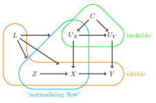
The following variables are part of the model:

• \(Z\), the instrumental variables (a vector of length \(d_Z\)).
• \(X\), the treatment variables (a vector of length \(d_X\)).
• \(L\), pre-treatment covariates (a vector of length \(d_L\)).
• \(Y\), the outcome variable (a scalar) which is either a binary variable or a continuous one.
• \(U_X\), hidden variables generating \(X\) (a vector of length \(d_X\)).
• \(U_Y\), hidden variable generating \(Y\) (a scalar).
• \(C\), hidden categorical mixture indicator taking values in \(\{1, \ldots, K\}\).

Vectors \(X\), \(U_X\) and \(U_Y\) contain only continuous variables.

The model is defined as follows.

Conventions

The model specification will involve several multilayer perceptrons (MLPs). We adopt the convention that for any MLP \(f_\alpha\) that is mentioned, it is implied that it comes with a structure of \(M_\alpha\) hidden layers and \(H_\alpha\) hidden units per layer, with model parameters \(\theta_\alpha\). We will write \(f_\alpha(\dots; \theta_\alpha)\) to denote the prediction/evaluation of the MLP, where \(\dots\) will be replaced with the data inputs to \(f_\alpha\) and \(\theta_\alpha\) denotes the MLP parameters that are being used. To save on space and notation, we will often leave implicit that \(f_\alpha\) depends on \(\theta_\alpha\), and simply write \(f_\alpha(\dots)\).

\(p_{\mathcal{N}}(\cdot; m, v)\) is used to denote the Gaussian density function with mean \(m\) and variance \(v\).

Instruments and covariates

Variables \(Z\) and \(L\) are always given as inputs for any data point, so there is no probabilistic model for them.

Hidden variables

The joint vector \((U_X, U_Y)\) is modelled using a Gaussian mixture model, defined as follows.

Let \(\pi_{ul}(c)\) be the probability mass function of a mixture indicator \(C\) taking value \(c \in \{1, 2, \dots, K\}\) given \(U_X = u, L = l\). Here, \(K\) is a hyperparameter of the model, assumed to be fixed. Define

\[\pi_{ul} \equiv \mathrm{softmax}(f_\pi(u, l; \theta_\pi)),\]

using the softmax function, where \(f_\pi\) is an MLP. \(f_{\pi}\) returns a vector of \(K\) entries, which is mapped by the softmax function to a vector whose entries are non-negative and sum to one.

Given \((C = c, Z = z, L = l)\), the conditional mean of \((U_X, U_Y)\) is defined to be zero for all \((c, z, l)\). We define the conditional covariance matrix of \(U_X\) to be the \(d_X \times d_X\) identity matrix, and the variance of \(U_Y\) to be 1. What is left to be modelled is the conditional cross-covariance between \(U_X\) and \(U_Y\),

\[ \sigma_{czl} \equiv \mathbb E[U_X U_Y \ \vert \ C = c, Z = z, L = l], \]

that is, \(\sigma_{czl}\) is the \(d_X \times 1\) cross-covariance vector. We parameterise it as follows:

\[ \sigma_{czl} = \mathrm{sigmoid}(f_m(c, z, l; \theta_m)) \times \frac{\tanh(f_r(c, z, l; \theta_r))}{\left\| \tanh(f_{r}(c, z, l; \theta_r)) \right\|_2}, \]

where

• \(f_r(c, z, l; \theta_r)\) is an MLP which outputs a \(d_X\)-dimensional real vector,
• \(f_m(c, z, l; \theta_m)\) is an MLP which outputs a real number.

Notice that the resulting cross-covariance vector has the squared norm

\[ \vert\vert\sigma_{czl}\vert\vert_2^2 = \sigma_{czl}^{\top}\sigma_{czl} = \mathrm{sigmoid}^2(f_m(c, z, l; \theta_m)) \lt 1, \]

and all entries lie in \((-1, 1)\). This is important, because we can write the conditional distribution of \(U_Y\) given \(U_X = u_x\), \(C = c\), \(L = l\), \(Z = z\) as

\[ U_Y \ \vert \ u_x, c, z, l \sim \mathcal{N}(\sigma_{czl}^{\top}u_x, 1 - \sigma_{czl}^{\top}\sigma_{czl}), \]

which is a valid distribution only if the squared norm of the cross-covariance is less than 1.

Model for treatment \(X\)

Let

\[ X = f_X(U_X, Z, L; \theta_X), \]

where \(f_X(U_X, Z, L; \theta_X)\) is a normalising flow feedforward network such that

\[ U_X = g(X, Z, L) \equiv f^{-1}_{X}(X, Z, L; \theta_X) \]

is the inverse of the flow on \(X\) for a fixed \(Z\) and \(L\).

Model for outcome \(Y\)

If \(Y\) is continuous, define

\[ Y = f_Y(U_Y, X, L; \theta_Y), \]

where \(f_Y\) is an MLP.

If \(Y\) is binary, let \(\tilde f_Y\) be an MLP and define

\[ \mathbb{P}(Y = 1 \mid U_Y, X, L) = f_Y(U_Y, X, L; \theta_Y) := \mathrm{sigmoid}\!\left( \tilde f_Y(U_Y, X, L; \theta_Y) \right). \]

Thus, in both cases

\[\begin{align} d(x,l) &:= \mathbb{E}\!\left[ Y \mid \operatorname{do}(X=x), L=l \right] \notag \\ &= \int f_Y(u_y,x,l)\, p_{\mathcal N}(u_y;0,1)\, \mathrm{d}u_y. \label{eq:causal-response} \end{align}\]

Notice that \(f_Y\) contains parameters of the model, here left implicit. Moreover,

\[\begin{align} r(x,z,l) &:= \mathbb{E}\!\left[ Y \mid X=x, Z=z, L=l \right] \notag \\ &= \int f_Y(u_y,x,l)\, p_{U_Y\mid U_X,Z,L}(u_y\mid u,z,l)\, \mathrm{d}u_y \notag \\ &= \int f_Y(u_y,x,l)\, \sum_c \pi_{ul}(c)\, p_{\mathcal N}(u_y;m_{c},v_{c})\, \mathrm{d}u_y. \label{eq:regression-model} \end{align}\]

where

\[ u := g(x, z, l), \quad m_{c} := \sigma_{czl}^\top u, \quad v_{c} := 1 - \sigma_{czl}^\top\sigma_{czl}. \]

Parameter and Hyperparameter Summary

To summarise, this continuous treatment model has the following parameters and hyperparameters.

Hyperparameters:

• \(K\), the number of mixture components, such that \(C \in \{1, \ldots, K\}\).
• Hyperparameters that are used to specify the feed-forward normalising flow \(f_X\), relating \(X\) to \(U_X\).
• \(M_{r}\) and \(H_{r}\), the hidden layer specifications for the MLP \(f_r\).
• \(M_{m}\) and \(H_{m}\), the hidden layer specifications for the MLP \(f_m\).
• \(M_{\pi}\) and \(H_{\pi}\), the hidden layer specifications for the MLP \(f_{\pi}\).
• \(M_{Y}\) and \(H_{Y}\), the hidden layer specifications for the MLP \(f_Y\).
• The numerical integration rule used to evaluate the regression function \(r\) and causal response \(d\).
• \(Q\), the number of quadrature points or Monte Carlo samples used by the numerical integration rule.

Parameters:

• \(\theta_{m}\), the weights and biases of the MLP \(f_m\).
• \(\theta_{r}\), the weights and biases of the MLP \(f_r\).
• \(\theta_{\pi}\), the weights and biases of the MLP \(f_{\pi}\).
• \(\theta_{X}\), the parameters specifying the normalising flow \(f_X\) and \(g = f_X^{-1}\).
• \(\theta_{Y}\), the weights and biases of the MLP \(f_Y\).

Note that \(\theta_X\) will be "learnt" during the initial learning stage, and held constant thereafter. We denote the entirety of model parameters as:

\[ \theta := \left(\theta_X, \theta_\pi, \theta_m, \theta_r, \theta_Y\right). \]

Learning and Querying

Assume we are given a dataset \(\mathcal{D}_{train}\) with training points \((z^{(i)}, x^{(i)}, y^{(i)}, l^{(i)})\). Use this to learn an estimate \(\hat{r}(x, z, l)\) of the regression function of \(Y\) on \((X, Z, L)\). For instance, XGBoost, random forests, TabPFN etc., can be used for that.

Moreover, fit a normalising flow to get \(\hat{\theta}_{X}\) using the training set.

To use the model, we are given a dataset \(\mathcal{D}_{eval}\) containing \(n_{eval}\) evaluation points \((z^{(i)}, x^{(i)}, l^{(i)})\). Let \(\hat{r}_i\) be the evaluation of the estimate of the regression function at data point \(i\) of \(\mathcal{D}_{eval}\).

Let \(r_i(\theta)\) be the evaluation of the regression equation \(r(x^{(i)}, z^{(i)}, l^{(i)})\) at parameter value \(\theta\), as given by \(\eqref{eq:regression-model}\). Here we are making explicit that this expression depends on all model parameters \(\theta\).

Learn initialiser

We will first learn some parameter value \(\theta^\star\) that is the minimiser of

\[\begin{equation} B(\theta) := \frac{1}{n_{eval}}\sum_{i \in \mathcal{D}_{eval}} (\hat{r}_i - r_i(\theta))^2. \label{eq:loss-function} \end{equation}\]

Using a gradient-based method with respect to some parameter \(\theta_j \in \theta\) means

\[ \frac{\partial B(\theta)}{\partial \theta_j} = -\frac{2}{n_{eval}}\sum_{i \in \mathcal{D}_{eval}}(\hat r_i - r_i(\theta))\frac{\partial r_i(\theta)}{\partial \theta_j}. \]

In practice, we approximate \(r(\theta)\) at any particular point by first standardising \(u_y\) for each mixture component \(c\),

\[ s := \frac{u_y - m_c}{\sqrt{v_c}}. \]

We choose a set of positions \(s_1, \dots, s_Q\) and weights \(w_1, \dots, w_Q\) to get

\[\begin{align} r(\theta) &= \sum_c \pi_{ul}(c) \int f_Y(s\sqrt{v_c} + m_c, x, l) p_{\mathcal{N}}(s; 0, 1) \mathrm{d}s \notag \\ &\approx \sum_{c=1}^K \pi_{ul}(c) \sum_{q = 1}^Q w_q f_Y(s_q \sqrt{v_c} + m_c, x, l). \label{eq:approx} \end{align}\]

As \(s\) by construction follows a standard Gaussian, two alternative choices for \(w_q\) and \(s_q\) are:

• (i) points and weights as given by Gaussian quadrature with \(Q\) points;
• (ii) \(Q\) Monte Carlo samples from a standard Gaussian with each \(w_q\) equal to \(1 / Q\). Here, \(Q\) is an algorithm hyperparameter that needs to be given as input.

When doing gradient-based optimisation of \(\eqref{eq:loss-function}\), we will keep \(\theta_X\) fixed at \(\hat{\theta}_X\). One way of interpreting this is by setting \(\partial B(\theta) / \partial \theta_j = 0\) for each component \(\theta_j\) of \(\theta_X\), with initialisation \(\theta_X = \hat{\theta}_X\). The other elements of \(\theta\) should be initialised at small values. If the Monte Carlo method is used, resample \(s_1, \dots, s_Q\) at each data point \(i\) at every iteration.

Ideally, \(B(\theta^\star)\) should be close to zero. Reporting its value to the user will allow them to identify issues, e.g., poor initialisation or poor choice of \(K\).

Query bounds on causal response

Learning is done once, but a user can query multiple causal bounds at various values of \(L\) and \(X\). In particular, we want lower bounds and upper bounds on \(\eqref{eq:causal-response}\) for some given \((x, l)\) as a function of \(\theta\).

For that, we need to solve two optimisation problems, maximise (for upper bounds) and minimise (for lower bounds) \(d(x, l; \theta)\) subject to

\[B(\theta) \leq B(\theta^\star) + \epsilon,\]

where \(\epsilon\) is a small number given by the user. Augmented Lagrangian methods can be used here. A hacky but potentially practical alternative is to directly optimise

\[ e(\theta) \equiv d(x, l; \theta) - \lambda B(\theta), \]

where \(\lambda\) is a penalty term that starts at zero and is increased until the optimisation reaches \(B(\theta) \leq B(\theta^\star) + \epsilon\). Increases take place at "small" steps once each optimisation converges for a fixed \(\lambda\), although what "small" is might require trial-and-error (which in one sense is what augmented Lagrangian optimisation methods adapt to).

The optimisation should start from \(\theta^\star\), and once again we keep \(\theta_X\) frozen at \(\hat{\theta}_X\).