Isobenefit Urbanism: QGIS Plugin

Exploring walkable urban growth on real-world data

The Isobenefit Urbanism plugin for QGIS simulates how a place could grow so that everyone keeps walkable access to both mixed-use local centres (shops and services among homes) and green space. From the simulation it generates idealised planning scenarios. It runs on your own GIS layers.

This is research software for discussion and debate. Its scenarios are speculative sketches of walkable growth in a place, made to be discussed with domain experts and weighed by them when developing actual planning strategies and developments. The scenarios are not plans to build from.

An idealised scenario for Cambourne: new settlements with walkable centres woven through a green matrix around the existing town — An idealised scenario for **Cambourne**, grown from the downloaded layers shown below. New settlements, coloured by density from pale (low) to deep (high), with their mixed-use centres in red, join the existing town (light purple), and new homes stay within a walk of a centre and of green. The same example is used throughout this page.

Concept & rationale

Isobenefit Urbanism (Luca D'Acci) describes a city whose benefits are spread evenly; the iso means equal. Wherever you live, and however large the settlement grows, you can walk both to a local centre and to green land, so quality of life does not depend on which part of town you live in. The aim is to avoid sprawl, which strands people far from centres and paves over nature, and equally to avoid overcrowding, which squeezes nature out.

It also sits between master-planning and laissez-faire growth: a few simple rules guide development, while the detailed form is left to emerge. The plugin works the same way. A cellular-automaton simulation grows a grid of land cells step by step under rules that keep new development within a walk of a centre and protect green corridors. The rules include randomness, so there is no single answer; the plugin runs many simulations and reports the variation across them, as well as coherent individual scenarios.

The settlements and their centres should also be linked by effective public transport (buses and rail). Without that link they would not work as one cohesive city, and dispersed development then indicates a problem. The plugin downloads streets, stops and stations for this purpose.

Using the plugin

This page explains the model, using one real town throughout. To install the plugin and run it yourself, the plugin guide covers installation, a first-run walkthrough, the run dialog, the outputs and troubleshooting. Ready-made places to start from, with data and parameters prepared, are in the scenario library.

Step 1: Download the data

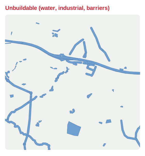
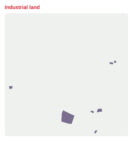
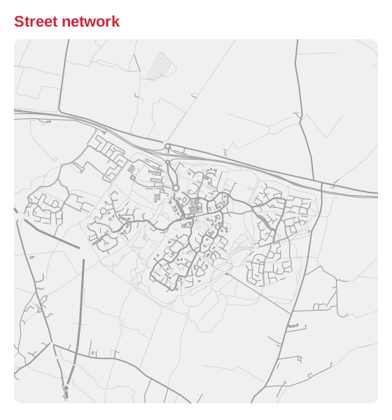
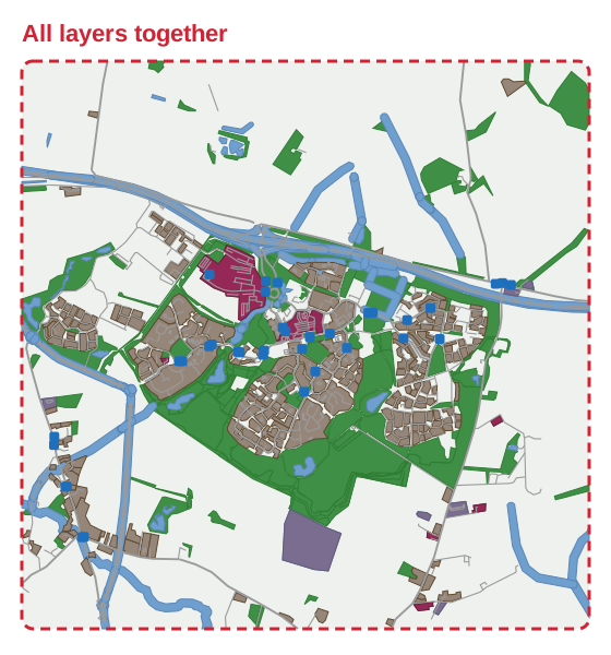
A companion Extract from OpenStreetMap tool downloads the input layers for an area of interest, so no manual data preparation is needed. The downloaded layers are ordinary editable layers, though: you can adjust them before running a simulation, or use your own layers instead. The panels below are the downloaded layers for a 4.2 km window around Cambourne, fetched with the plugin's own queries. Each panel shows one layer of the same place. The layers partition the town: green does not overlap built land, centres sit inside the built fabric, and stacked together they add back up to the whole town.

The extents layer sets the area of interest. It is the only layer the simulation requires.

The existing built fabric. The simulation treats it as fixed and never redevelops it.

Existing green space, which the growth rules preserve.

Mixed-use urban centres, taken from retail and commercial land. Every cell they cover acts as a centre.

Unbuildable land: water, industrial land, and buffered barrier corridors such as the A428.

Industrial land. It stays as it is, but no new housing is placed on it.

The street network, classed by road type. It gives the maps their context, and its major-road corridors (motorway, trunk and primary) are carved as barriers.

Public-transport stops. Bus stops act as growth anchors: with the corridor preference raised, development concentrates within their walkable catchment. Rail and tram stations act as centre anchors, seeding growth and pinning a centre.

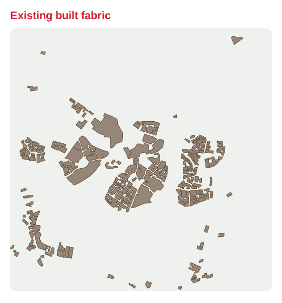
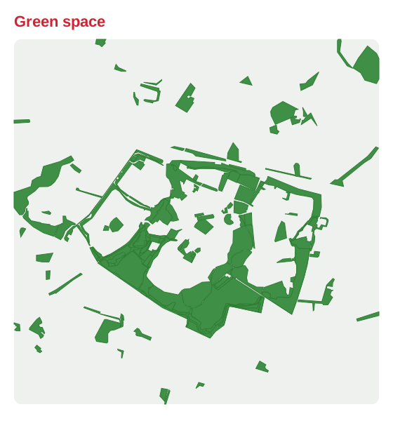
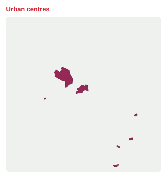
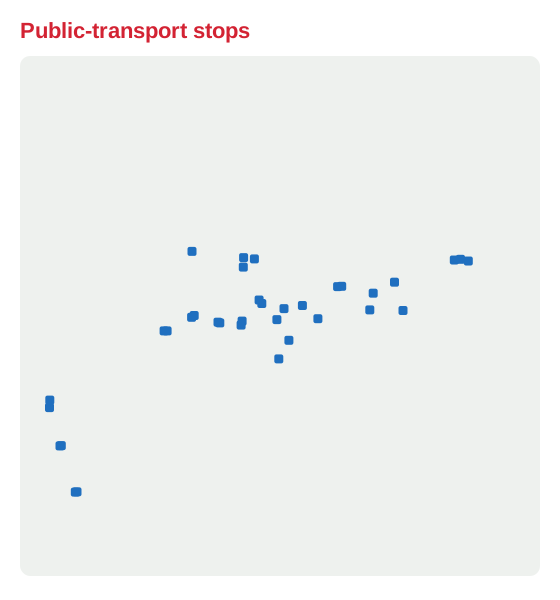
Two further datasets, railways and rail/tram stations, are also downloaded. They are empty here because Cambourne has no railway. Where stations do exist, they seed growth and anchor centres in the scenarios. The two transit layers give a planner direct transit-oriented levers: a point added to the hubs layer places a designated centre, a station for a planned line for example, while a proposed bus corridor drawn as a line steers growth along it once the corridor preference is raised above 0.

All downloaded layers stacked into one map of Cambourne — All of the layers together. Throughout this page, vector shapes show *data* and dots show the *simulation*.

Step 2: From layers to cells

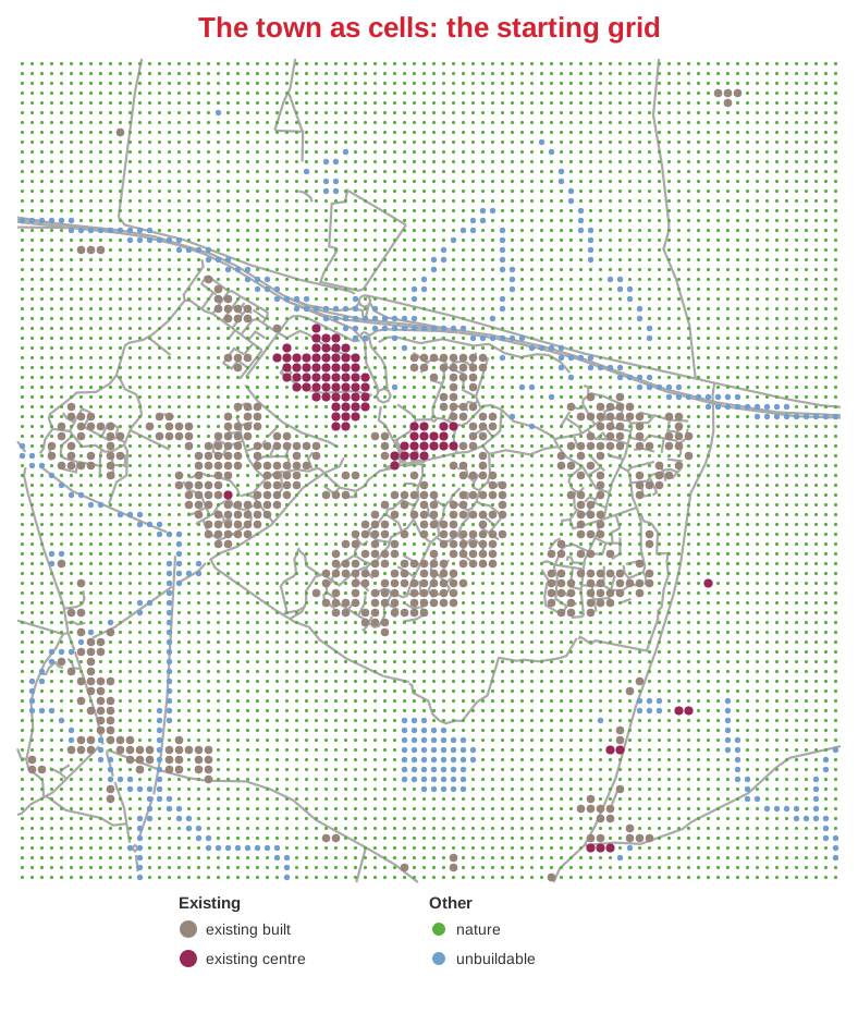
In QGIS you point the run dialog at these layers, choose a projected CRS and an output path, and press Run; the rest is automatic. The simulation works on a grid (here 50 m cells), so the vector layers are rasterised first: existing built fabric becomes fixed built cells, downloaded green becomes protected green cells, centre areas become centre cells across their full extent, and water, industrial land and buffered barrier corridors (major roads, railways, rivers) are marked unbuildable, so the simulation never develops them. Where a pedestrian-navigable road or footpath crosses an unbuildable corridor, that cell is marked walkable instead: still never developed, but a walk may pass through it, so a footbridge or level crossing keeps access viable across a railway or river rather than the corridor severing everything beyond it. The walkable ways come as their own downloaded layer, so crossings can be edited from local knowledge. Every run on this page starts from this grid:

Cambourne rasterised to the simulation grid — The town as cells. The brown dots are the existing built fabric, the black dots its existing centres, the blue dots water, and the grey dots other unbuildable cells; the A428 corridor and the waterways stand out. The small green dots are free land, and the real street network stays visible beneath.

Step 3: The simulation

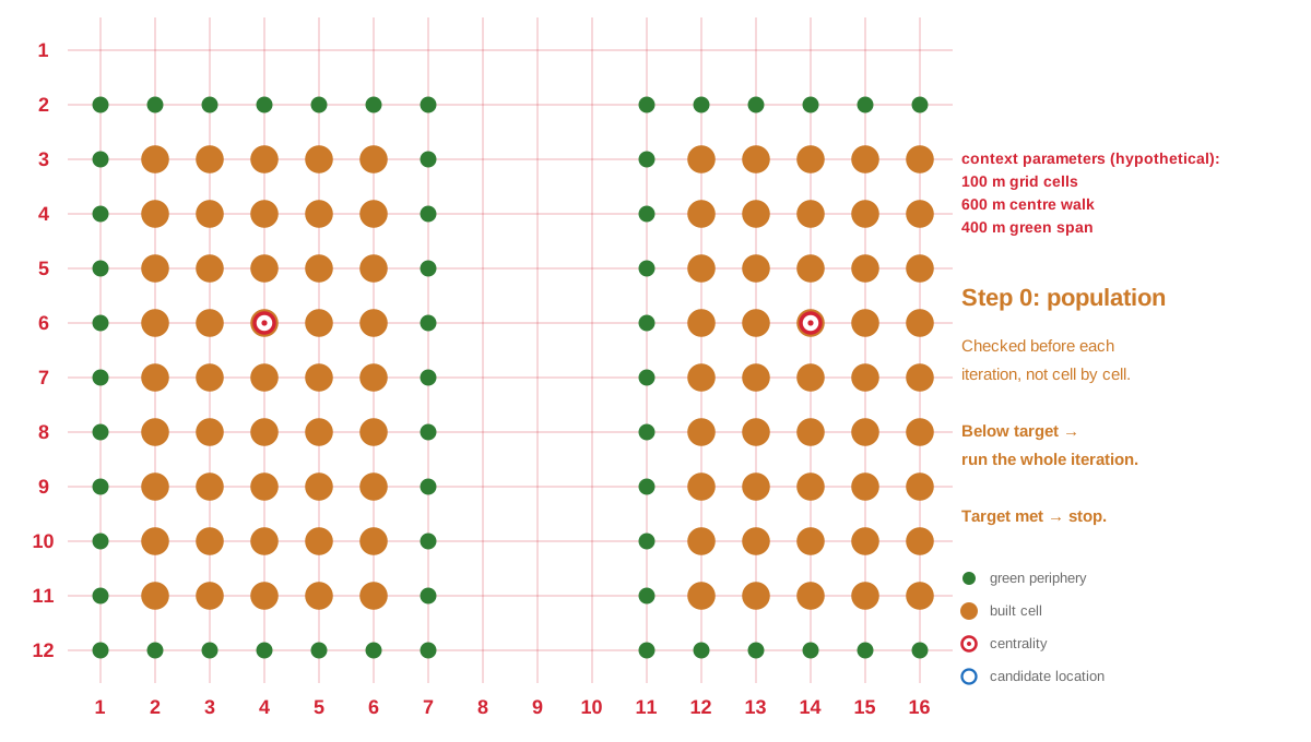
Each step, the cellular automaton visits the land grid and decides whether an undeveloped cell may be built. The rules are shown below, zoomed into a schematic neighbourhood.

Step 0: population target

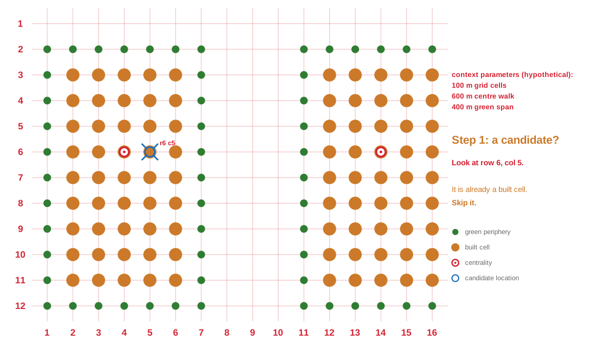
Step 1: a candidate cell

A cell is only a candidate if it is empty and on the periphery of built land:

This cell is already built, so there is nothing to do and it is skipped.

This cell is empty but touches no built land, so it is not on the periphery and is skipped.

This cell is empty and touches built land, so it is a candidate and the checks continue.

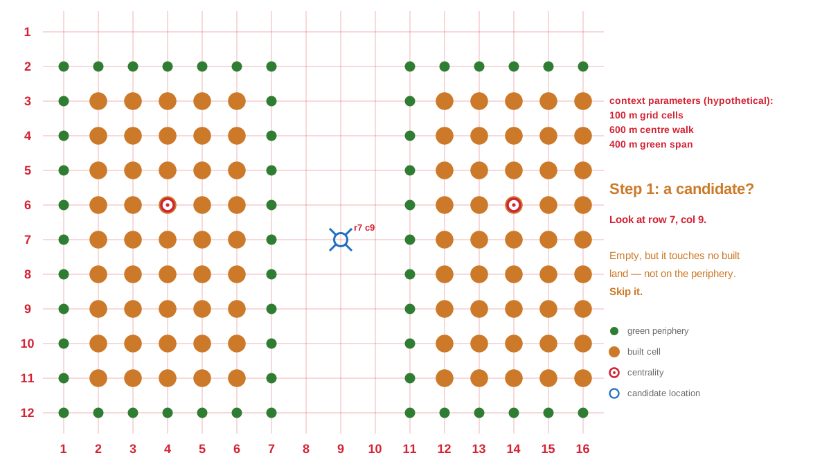
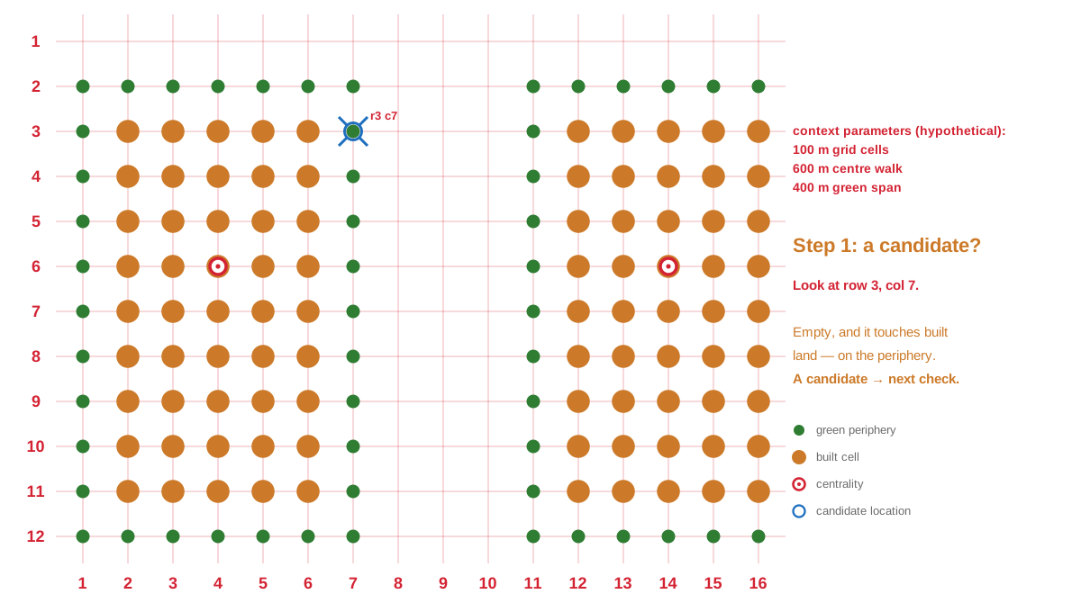
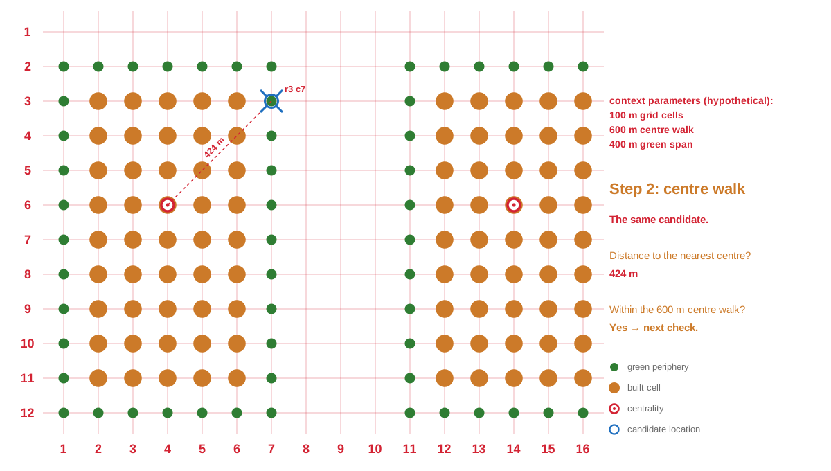
Step 2: centre walk

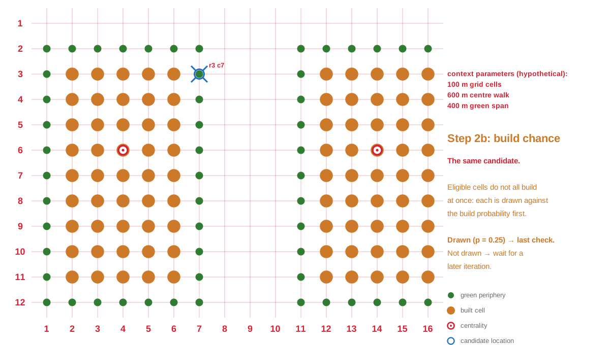
Step 2b: build chance

Step 3: green span

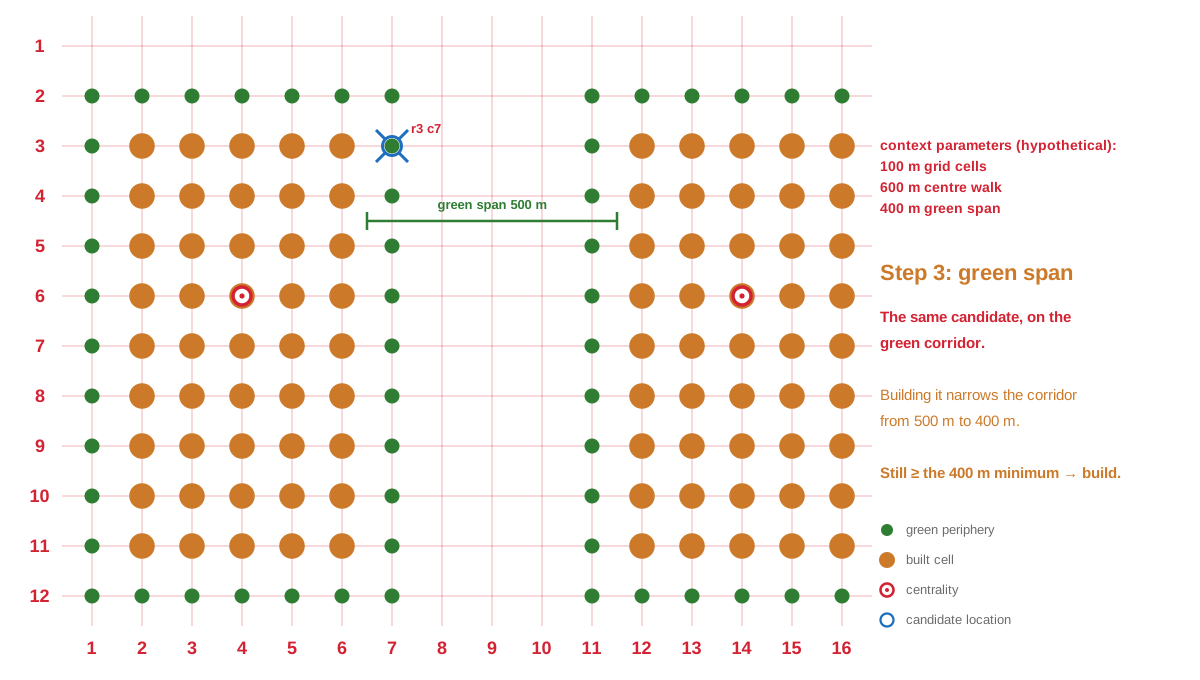
Step 4: build

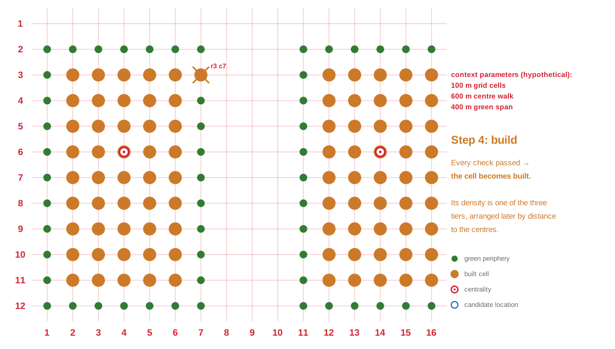
Two green settings play different roles. The minimum green span above is a building rule; the simulation refuses to pinch a green corridor below that width. The green walk sets how far a home may be from usable green, and it is judged on the finished scenario alongside the centre walk.

Where new centres come from

As built land grows to the edge of the centre walk, frontier cells just beyond it can no longer build. Each such cell has a small fixed chance (1% per iteration, at most one new centre per iteration) to seed a new neighbouring centre, which lets a single town keep growing outward. A separate setting, Dispersed development (Off, Moderate or Aggressive), sets the chance that a far-off green cell instead seeds an isolated centre, so development leapfrogs away from the core to form satellite settlements. Both centre draws are probabilistic, like the build chance, and the Random seed makes any run repeatable.

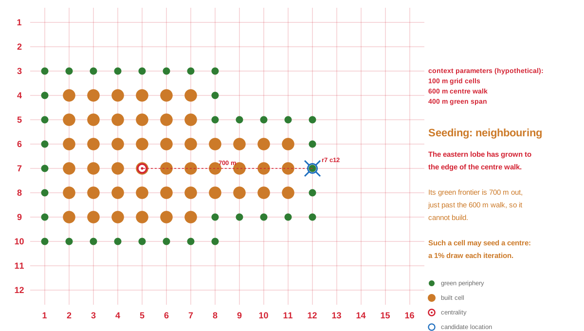
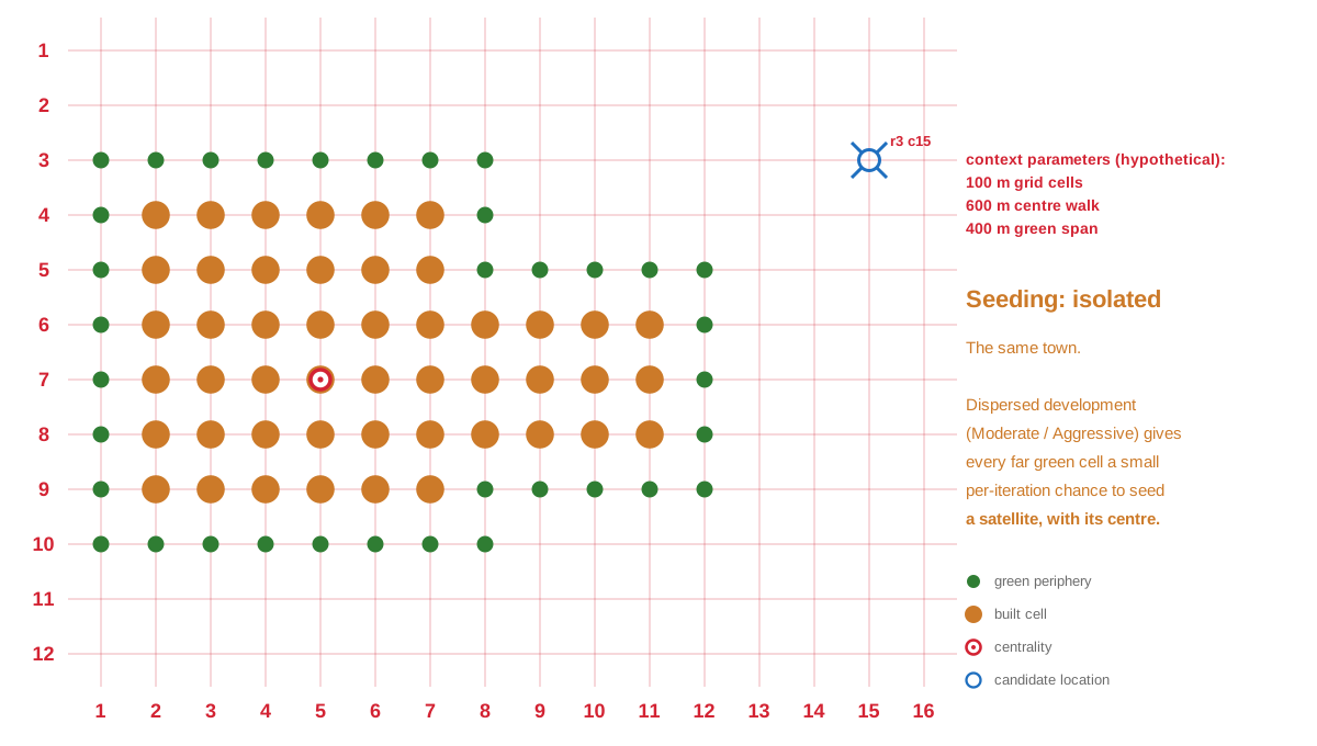
A neighbouring centre may seed where the frontier sits just past the centre walk: at 700 m here, since growth stops at the walk's edge.

The same town: an isolated centre lets a satellite settlement leapfrog away from the core, at the rate set by Dispersed development.

The rules at work on the real town

Below, those rules run on the Cambourne grid from step 2; the three figures show the same run at three points in time. New development (coloured by density) stays on the periphery of the existing fabric, keeps within a walk of a centre (red seeds appear as the town outgrows them), and does not build on the green corridors or the unbuildable cells.

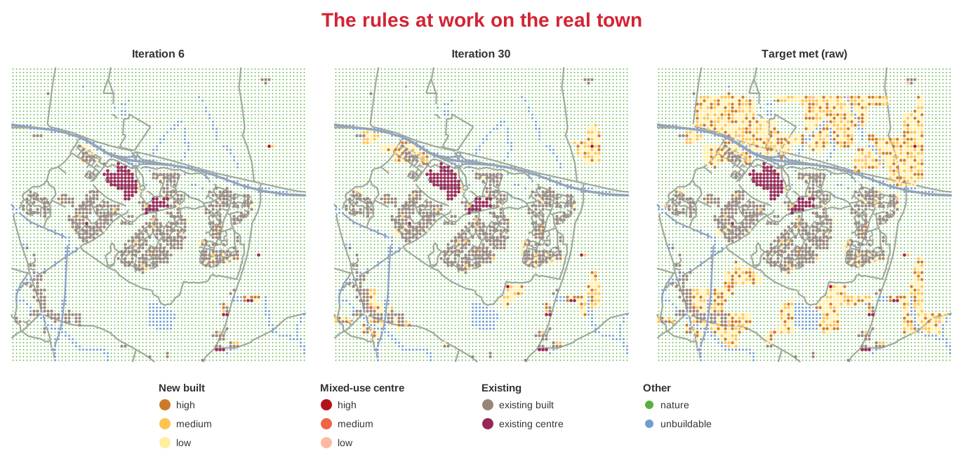
The growth rules at work on Cambourne, at iterations 6 and 30 and once the target is met — The same run at three points: first infill at the edges (iteration 6), settlements consolidating with new centres seeded (iteration 30), and the raw grown state once the target is met.

Two further settings shape growth. The build probability is the per-step growth rate; lower values give compact growth, higher values looser growth. The development density is set as three tiers (low, medium and high, each a density in people per km²), each with a share, and the three shares sum to 1. Every new cell is built at one of the three densities, drawn at those shares, so the shares set the mix. Growth counts new development only, and stops once the new population reaches the target; the existing fabric is context and is not counted. Counting it would demand inputs that rarely exist in practice: a reliable population for every existing block, and the capacity of every existing centre. Treating existing fabric as already-served context needs neither. The finished scenario then arranges the drawn densities and colours the result by tier, described in step 5.

Step 4: From many runs to one scenario

A single run is one plausible outcome; a different random seed gives a different, equally valid layout. So the plugin runs an ensemble and does two things with it. First, it blends the runs into a development-likelihood map; the map below blends 24 runs over Cambourne.

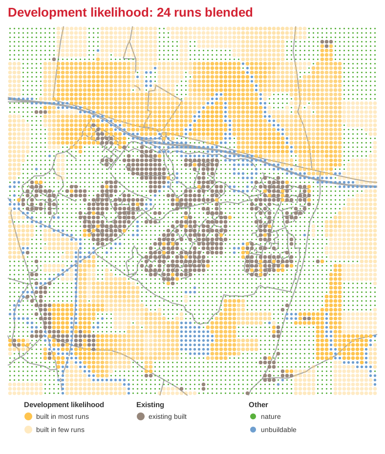
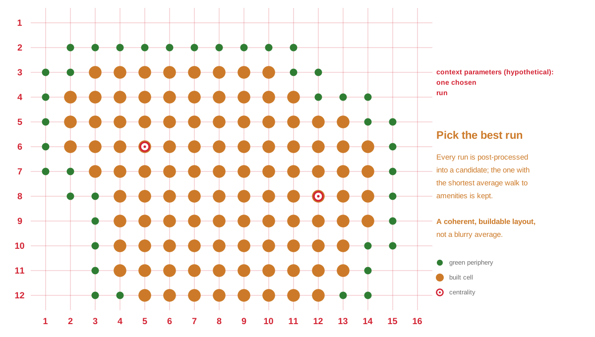
Development likelihood over Cambourne from 24 blended runs — Each cell's shade is the share of runs in which it ends up built: dark where most runs build the cell, faint where few do.

Because a probability surface is not a buildable layout, the plugin also produces one buildable scenario. Every run in the ensemble is first post-processed into a candidate (the edits are described in step 5), the candidates are scored, and the one with the shortest average walk to amenities is kept.

Every run is post-processed and scored; the winner becomes the scenario and the others remain in the likelihood map.

Step 5: Post-processing the runs

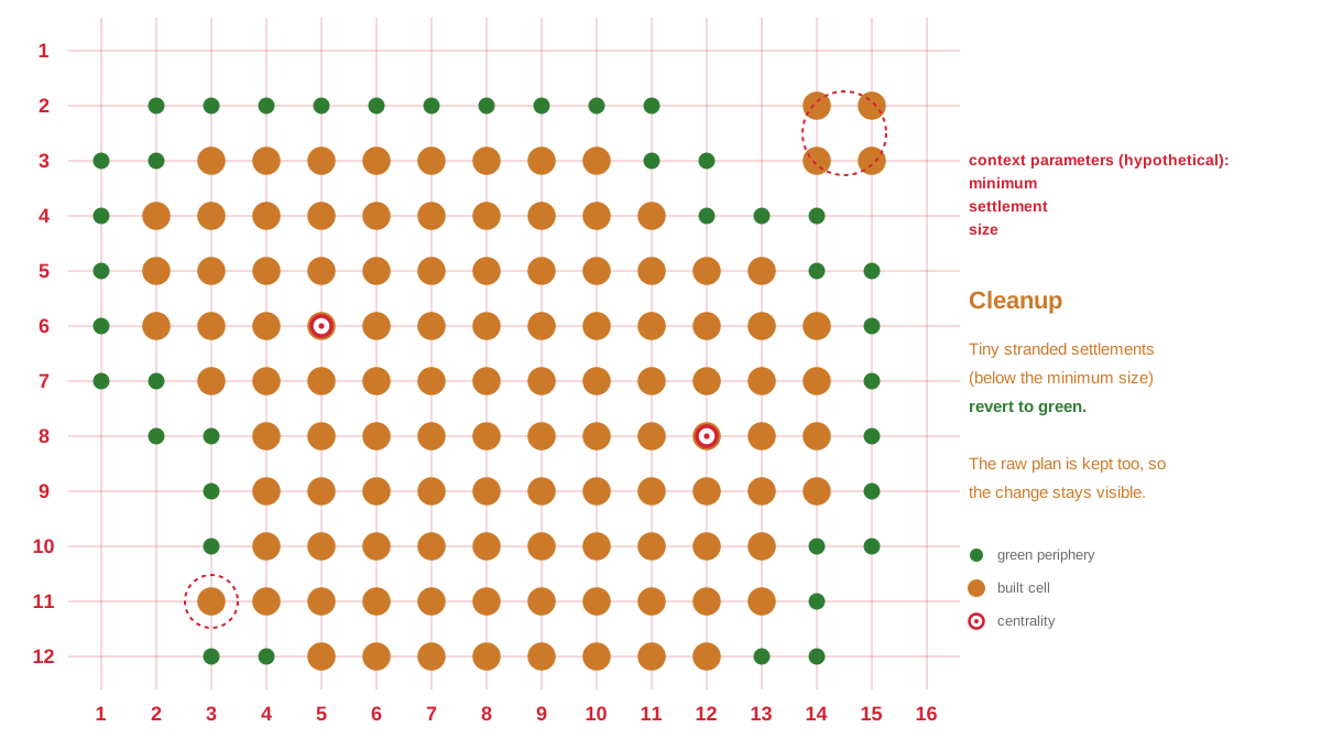
Each run is refined into a candidate scenario before the scoring in step 4; the winner is the scenario the plugin loads. Post-processing changes the centres and applies a limited building cleanup; the buildings themselves come from the simulation.

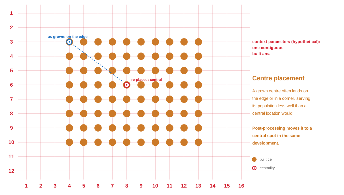
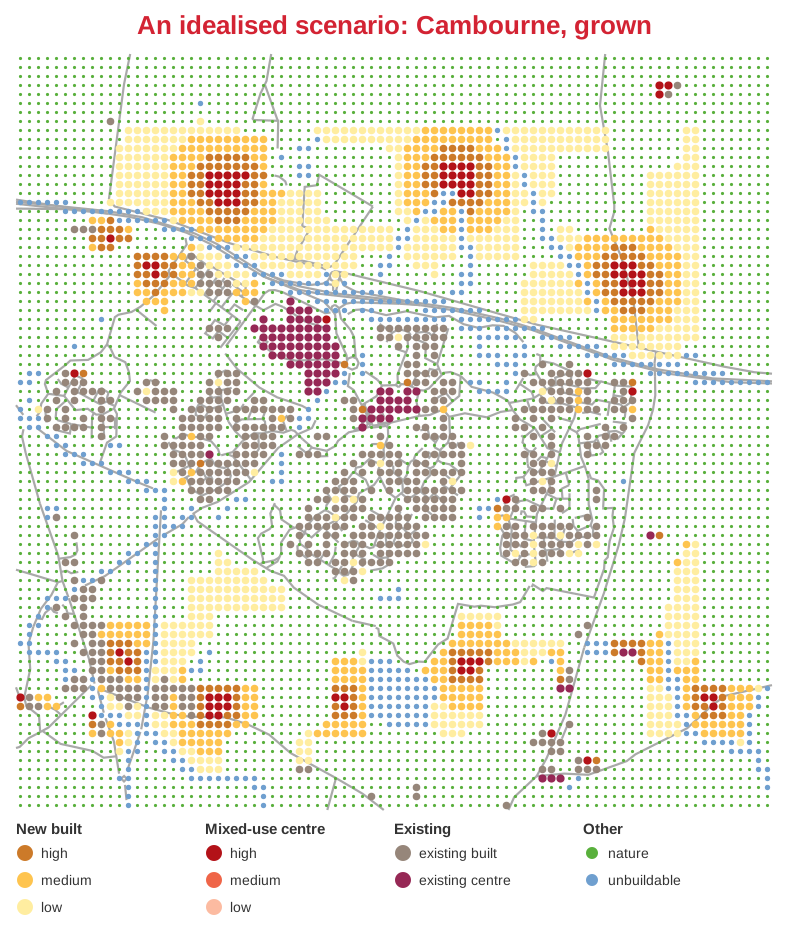
In the cleanup, growth that no viable centre reaches reverts to green.

A grown centre often lands on the edge or in a corner of its development, so it serves its population less well than a central location would. Each is moved to a central spot in the same built area.

The centres are mixed-use throughout: a centre cell keeps its homes and gains shops and services, and each centre is sized by the population it serves at a rule-of-thumb provision (m² of centre land per person). Where new development has no centre of its own within a walk, one is added. An existing centre nearby serves the existing town and any small infill within its walk, while a real new district still earns its own centre, so development cannot sprawl centre-free along existing fabric. Once the centres are settled, each scenario is coloured by density tier. The densities drawn during the run are arranged by walking distance to the final centres: the highest sit nearest a centre, then medium, then low. The mix of tiers is fixed, so the total population does not change; only their placement is set here. Arranging it after post-processing, rather than during growth, means the placement is measured against the centres the scenario actually shows, not against whichever centres happened to exist mid-run.

This centre-and-density arrangement is also what makes public transport workable. A well-placed mixed-use centre, with the densest housing gathered around it, concentrates residents, shops and services in one walkable catchment; a bus or tram stop at the centre then serves the most people and the most destinations per stop. Scattered centres and flat densities spread that demand too thin for a service to run frequently.

Finally, centres are offered as options. The run and the buildings are the same; only the centre treatment differs: as grown keeps the centres where the run grew them, optimised placement re-positions them to cut walking distances, and fewest centres also removes any centre whose loss leaves no home beyond the walk. Every option keeps the model's hard rule: no home further than the centre walk from a centre. Under low growth pressure the placed and fewest options come out the same, and that is expected: a small settlement needs its few centres wherever they sit. They separate once settlements grow large enough to hold redundant centres, so the comparison below is grown to a 20,000-person target rather than the worked example's 12,000.

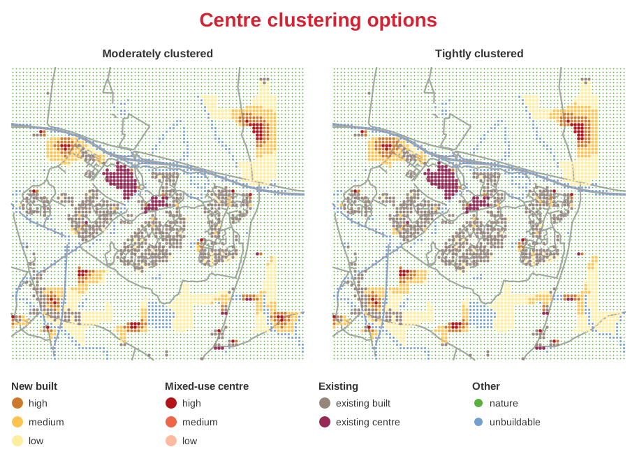
Two centre options for the same run: optimised placement and fewest centres — The same run and buildings under two centre options: optimised placement keeps the run's centres and walks each central to the homes it serves (555 m average walk here, counted over every home); fewest centres also removes any centre whose loss strands no home, consolidating provision into fewer, larger centres (567 m average). The built cells are identical; the density tiers re-arrange around whichever centres remain, and no home ends beyond the centre walk of one.

Either can be compared against the raw grown state at the end of step 3. The raw state is always saved alongside, so the effect of post-processing stays visible.

Step 6: Outputs

An ensemble run writes a small set of layers, each shown above:

existing development, the starting grid from step 2
raw (before post-processing), the chosen run as it grew (the end of step 3), coloured by the densities the run drew in place
centres as grown, optimised placement and fewest centres, the scenario options from step 5, each coloured by arranged density tier
development likelihood for built and for green, the uncertainty map from step 4
rejected development, a diagnostic layer mapping the raw growth the plans rejected, coded by reason (a satellite below the service viability threshold, or growth in a centreless hamlet), so the difference between the raw run and the options explains itself
_report.txt, a record of the parameters and the per-option statistics

Reading the report: every population figure counts new residents only. Existing fabric is shown for context and is assumed to be served by its own centres, so it is never counted. The per-person readouts follow the same convention: m² of centre per person is new mixed-use centre land over new residents, and m² of walkable green per person is new green over new residents. Coverage is reported twice: over new homes, where the growth rules guarantee a centre and a park within the walks, and including every existing home, which carries no guarantee.

A single run, with the ensemble checkbox off, is instead written step by step as a growth animation you can play in the QGIS Temporal Controller. The three growth moments in step 3 are three such frames.

The figure at the top of the page is the optimised-placement scenario from this pipeline.

Changing the parameters

Every figure below is a run on the same Cambourne grid; only the named parameter changes between figures.

Dispersed development

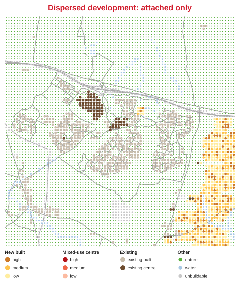
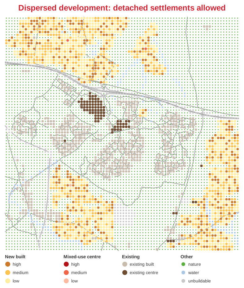
This control sets where a centre may go once growth has earned one: attached to development that already exists, or detached from it. It also sets how much of the population target fits, because a detached settlement opens land that edge-only growth can never reach within the walkability rules. Both panels show the raw grown state, before post-processing.

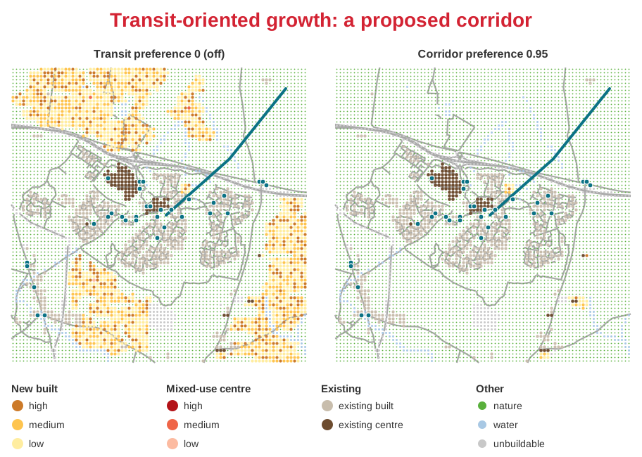
Attached only. Every earned centre must join existing development, so the town grows outward as one contiguous settlement.

Detached allowed. An earned centre may start a settlement away from the town, so growth reaches land the existing centres cannot serve.

Transit-oriented growth

The corridor preference concentrates development along public transport. The bus stops and any proposed route drawn as a line project a walkable catchment, 400 m by default, transit hubs project a wider one, 1,200 m by default, and outside those catchments every development draw is scaled by one minus the preference. At 0 the transit layers only feed the run report; at 0.95, as on the right, growth strings along the drawn route. The two panels share every other setting and show the raw grown state. A hub does more than project its catchment: it anchors a mixed-use centre that seeds growth and survives post-processing, so a point added to the hubs layer places a designated centre by hand.

The same Cambourne run with the corridor preference off and at 0.95: with the preference raised, growth concentrates along the proposed bus route — The teal line is a proposed bus route, drawn by hand; the teal dots are the downloaded bus stops. With the preference raised, growth gathers along the route instead of spreading evenly. The Cambourne entry in the scenario explorer runs the same demonstration at the full study window, with a proposed bus rapid transit stop anchoring a new settlement at the route's southern end.

Service viability

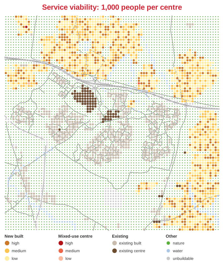
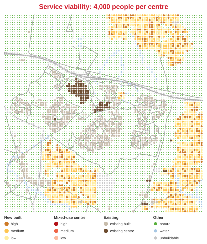
This is the population a centre must gather before growth earns the next one, so it sets how large the settlements become. Raising it yields fewer, larger settlements whose homes walk further to a centre; lowering it yields more, smaller ones. Because centres are earned rather than drawn, this figure decides how many the plan contains, whatever the size of the window or the resolution of the grid. Both panels show the raw grown state.

1,000 people per centre. More centres, each serving a smaller settlement.

4,000 people per centre. Fewer, larger settlements, with longer walks to a centre.

Departures from standard Isobenefit Urbanism

The growth rules themselves (periphery-only development, a walk to the nearest centrality, protected green spans, stochastic seeding of new centralities) follow D'Acci's morphogenesis and Voto's original simulator. Around that core, this implementation departs in several ways. The theory page gives the detailed comparison with the published model.

Ensembles instead of a single run. The original simulator produces a single run. The plugin runs many, blends them into likelihood layers, post-processes every run, and keeps the one with the shortest average walk to amenities.
Post-processing of the grown runs. The original keeps centres where they seeded. The plugin adds a limited cleanup (growth no viable centre reaches reverts to green) and offers centre options that all keep every home within the centre walk: as grown, optimised placement, and fewest centres, each sized by the population in its catchment at a m²-per-person rule of thumb. The raw grown state is saved alongside.
Density tiers arranged core-out. The original draws each block's density randomly from three fixed tiers, scattered across the map. The plugin keeps the three tiers and their shares, but arranges the drawn densities in post-processing so the highest occupy each settlement's interior core, then medium, then low toward the edge, with the walk to the mixed-use centres breaking ties. Gathering the densest housing at the core is what lets public transport work: a stop at a well-placed centre serves the most people and destinations. The mix is unchanged, so the population is the same; only the placement is organised. Growth counts new development only.
Walking distances rather than radii, one per amenity. The original measures straight-line distance within one walkable radius of roughly a kilometre (a 15-minute walk; D'Acci's later summaries use 1 to 2 km). The plugin measures a bounded walk over the grid that cannot cross unbuildable land, gives centres and green each their own distance, and defaults to 1,200 m for centres (a fifteen-minute walk, close to the published radius) and 400 m for green (the stricter everyday-green reach of the WHO and Natural England standards); both are settings the user can change.
Green connectivity is enforced locally rather than globally. The published model keeps all nature as one connected region. Real landscapes arrive already fragmented by rivers, roads and towns, so that rule cannot hold on real data. The plugin instead refuses to pinch a green corridor between developments below the minimum green span and, where new development would split green, requires each resulting fragment to keep at least the minimum park area. A green strip bounded by water or a carved road corridor is exempt from the span rule: it is not a corridor between developments, and land beside a barrier may be built right up to it.
Centres are earned, not drawn. The published model seeds centralities by probability, and a probability is meaningless to the person setting it: nobody can defend 0.005 over 0.01 from a map, and the same value yields a different number of settlements as the window, the cell size or the pace of growth changes. This implementation replaces those draws with a ratio a planner can actually interpret: each new home is charged to the centre it is nearest, and a centre founds the next one once that population reaches the service viability threshold (people per centre), or once it has no room left to grow. How many people a local centre must serve to be viable is a planning judgement with published reference points, the number of settlements follows the population rather than the grid, and a candidate whose only built neighbour is not a centre still may not build (which suppresses one-cell tendrils).
Real-data grounding. Existing fabric is fixed (never redeveloped); water, industrial land and barrier corridors (major roads, railways, rivers) are carved out as unbuildable, and a cell where a pedestrian-navigable way crosses a corridor is marked walkable, never developed but open to walks, so access stays viable across a bridge or level crossing; downloaded centre areas act as true multi-cell centres; and an OSM extraction tool supplies all of it. Rail and tram stations anchor centres; stops feed the report's transit readout. The growth rules and the scoring both measure bounded walks over the grid, blocked by unbuildable land. Street-network distances were tried and removed, since a new settlement's streets do not exist yet and a network metric would measure new and existing fabric on different terms.

Credits & sources

Based on the Isobenefit Urbanism concept by Luca D'Acci, with original Python code by Michele Voto. Developed as part of the Future Urban Growth project at UCL Bartlett School of Planning (Tommaso Gabrieli, Luca D'Acci, Heeseo Kwon, Stephen Marshall, Valentina Marin Maureira, Gareth Simons). The code lives at BSP-isobenefit-qgis-plugin.

Map data © OpenStreetMap contributors, available under the Open Database License (ODbL). Slope layers in the scenario library are derived from the Copernicus GLO-30 digital elevation model: produced using Copernicus WorldDEM-30 © DLR e.V. 2010–2014 and © Airbus Defence and Space GmbH, provided under COPERNICUS by the European Union and ESA; all rights reserved.

The plugin and its simulation engine are free software under the GNU AGPL-3.0-or-later. Problems and suggestions are welcome on the issue tracker.