Some useful details about the UKCP18 dataset
This is a quick reference guide to the data we’ll be looking at during the hackathon - feel free to ask the organisers if you have any questions that aren’t covered here.
First, some important things you need to know about the UKCP18 projections:
- they use a 360-day ‘year’, consisting of 12 months each with 30 days.
- seasons are defined as Winter (December-January-February, abbreviated to DJF); Spring (March-April-May, MAM); Summer (June-July-August, JJA); and Autumn (September-October-November, SON)
- the meteorological ‘year’ starts on December 1st (the beginning of winter) and ends on November 30th (the end of Autumn). So for example, the year 2021 starts on December 1st 2020 and finishes on November 30th 2021.
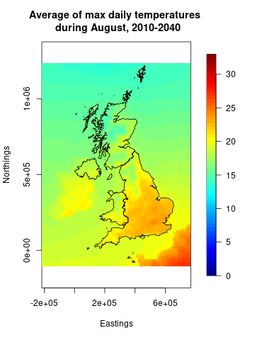
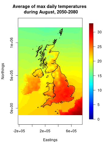
- The 12km projections are provided on the Ordnance Survey (OSGB) grid from Eastings -210000 to 762000 and Northings -102000 to 1086000 - you can see this spatial extent in the plots below.
- the full set of UKCP18 projections consists of 12 ensemble members, each using slightly different initial conditions and slightly different model physics. The data provided here is for ensemble 01, the ‘control’ run.
These example plots (produced using R) show the area covered by this data.


Which variables are available?
The UKCP18 data set consists of projections of 15 core variables under the RCP8.5 (high emissions) scenario:
| Variable name | Definition | Units |
|---|---|---|
| clt | Total cloud cover | % |
| hurs | Relative humidity at 1.5m | % |
| huss | Specific humidity at 1.5m | g/kg |
| pr | Precipitation rate | mm/day |
| prsn | Snowfall rate | mm/day |
| psl | Pressure at sea level | hPa |
| rls | Net surface long wave radiation flux | w/m2 |
| rss | Net surface short wave radiation flux | w/m2 |
| sfcWind | Mean sustained wind speed at 10m | m/s |
| snw | Lying snow | mm |
| uas | Eastward wind at 10m | m/s |
| vas | Northward wind at 10m | m/s |
| tas | Mean air temperature at 1.5m | °C |
| tasmax | Maximum air temperature at 1.5m | °C |
| tasmin | Minimum air temperature at 1.5m | °C |
The JupyterLab data science platform contains files with daily, monthly, seasonal, annual and 30-year averages of these variables, at a spatial resolution of 12km over the UK. The data can also be downloaded directly from the CEDA archive, but you will need to register for an account first.
Daily averages of two additional variables are also provided:
| Variable name | Definition | Units |
|---|---|---|
| sfcWindmax | Maximum sustained wind speed at 10m | m/s |
| wsgsmax | Maximum wind gust speed at 10m | m/s |
Both this and the three-hourly data required for the shipping forecast project can be found in ~/UKCP18/ukcp-other on the data science platform.
How do I know which file to use?
The filenames of the UKCP projections provide a lot of information about the data they contain. The structure is always the same:
<variable name>_<scenario>_<model>_<domain>_<spatial resolution>_<ensemble member>_<temporal resolution>_<start date>-<end date>.nc
- variable name will be one of the variables in the table above.
- scenario refers to the relative concentration pathway (RCP) used to run the simulations. All UKCP18 regional projections use RCP85.
- model refers to the model used to produce the projections. This hackathon is focussing on the regional projections over the UK land mass, which are output by the
land_rcmmodel. - domain denotes the geographical region of the data: projections are available over the whole of Europe, but the hackathon is targetting the UK projections.
- spatial resolution defines how the data are aggregated. The OSGB grid is at 12km resolution, but the Met Office also provide the data aggregated by country, administrative region, and river basin.
- ensemble member is denoted by a two-digit number. The full UKCP18 ensemble has twelve members; only data for the first is provided.
- temporal resolution: the data may be averaged over each day, month, season, or year. Daily, monthly, seasonal and yearly averages are also provided for thirty-year blocks.
- start date and end date are the first and last dates in the file.
The same elements are used to define the directory structure of the data in the CEDA archive - so if you want to download more data, you know how to find it.
Additional data
Teams are strongly encouraged to combine the UKCP18 projections with other data sets that might give useful insights. A few additional sources of data are provided on the data science platform:
Met Office shapefiles
The country outlines in the plots above are provided in ~/UKCP18/ukcp-spatial-files/spatial-files on the data science platform, or can be downloaded directly from github. The Met Office provides a large number of different shapefiles at various resolutions.
- ukcp18-uk-land-country-united_kingdom-hires contains the borders of the UK
- ukcp18-uk-land-country-hires contains the borders of the UK, and the internal borders between Wales, England and Scotland (this is the shapefile used in the plots above)
- ukcp18-uk-land-river-hires contains boundaries of river basins
- ukcp18-uk-land-region-hires contains boundaries of administrative regions (counties)
Examples of how to read shapefiles in R and Python are provided in Jupyter notebooks on the data science platform.
Land surface mask
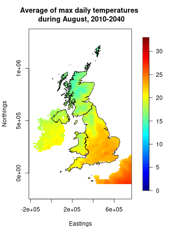
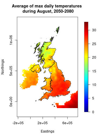
If you only want to plot the data over the UK land mass, you can use a land/sea mask to set all grid cells centred over water to a missing value. The Met Office’s land/sea mask is provided on the data science platform at ~/UKCP18/ukcp-other/land-sea_mask_uk_12km.nc.
Multiplying the data by the mask will produce plots like these:


Population projections
Researchers from NCAR’s IAM group and the City University of New York Institute for Demographic Research have developed a set of global, spatially explicit population scenarios that are consistent with the new Shared Socioeconomic Pathways (SSPs). The SSPs describe alternative future pathways of societal change that were developed to facilitate global change research, with SSP5 corresponding most closely to the RCP8.5 scenario modelled by the UKCP18 projections. A copy of the SSP5 population projections on the OSGB grid is available on the data science platform at ~/UKCP18/population/. The original data was produced on a slightly different grid, so we’d recommend using the prepared version.