 Close
Close

Common Data-Structures
There are some key data-structures with which you will need to be familiar. Each of these is a kind of container; we shall consider how these structures affect how we can access and insert data. We will discuss the complexity of data access and insertion for some of these in class.
Random Access Arrays
A random access array is the kind of array with which you are already familiar. Data is laid out sequentially and contiguously in memory, and so it is easy to calculate the memory location of any given element from the starting memory location and the index $i$ of the element. This is why they are called random access: we can access any element of the array in $O(1)$ time and no elements are harder to find than any others. Inserting an element into a random access array is often cumbersome due to the need to keep the data contiguous: if you want to insert data somewhere other than the end of the array then you need to shift all elements that appear afterwards in memory. This operation is $O(n)$.
std::vector, std::array, and C-style arrays are all examples of random access arrays.
In detail: std::vector in C++
The most common form of random access array that we use in C++ is std::vector, so it’s worth understanding a bit more about how it works. std::vector comes with operations to insert and remove elements, and it distinguishes between insert/removal in the middle of the vector and at the end.
Time complexity of push_back and pop_back
To add an element at the end of an array we can use push_back. To understand this operation’s behaviour from a complexity point of view, we have to think about the way that vector allocates and manages memory. A vector will allocate memory on the heap for its elements, and it will often allocate more memory on the heap than it needs to store its elements. It has separate data members to keep track of the size of the vector (i.e. the number of elements), and the size of the allocation. If the allocation is larger than the current size of the vector, then push_back(x) can simply place x in the next address in memery and increment the size counter. If however the allocation is full, a new, larger, allocation will need to be made and the entire array of data copied over to the new allocation in order to have space to add another element. (The previous allocation is then freed.) This means that some push_back operations take much longer than others, and as the vector gets bigger the time for this copy keeps getting larger! Just how much bigger the allocation should be made each time can have a significant impact on how the structure performs: std::vector uses a strategy that guarantees that the average (amortised) time for a push_back operation remains $O(1)$. (This is because although the time for a reallocating push_back keeps increasing as the array gets larger, the frequency of these operations goes down. For example, if you double the size of the allocation each time you reallocate, push_back will have amortised constant time.)
Although push_back takes amortised constant time, some push_back operations will take longer than others, which may be a concern if you have latency restrictions. Because of the reallocations and the need to check the size of the existing allocation, repeated push_back operations carry some overhead compared to simply setting the values within a vector. As such, when the size of the vector needed is known ahead of time, it is better to initialise a vector of the correct size and then set the elements in a loop rather than using push_back inside a loop. Using push_back can be the most natural approach however when this is not possible, for example streaming data in from a file where the total number of elements is not known.
There is a corresponded operation for removing an element from the end of the list, pop_back, which is always constant time since it cannot trigger a reallocation.
Insertion and removal of arbitrary elements
We also have insert and erase for inserting and removing elements. Removing elements will not require any reallocations, but it does require shifting any data to the right of the elements being deleted. Removing an element is therefore, on average, $O(n)$. Inserting an element works similarly, as it needs to shift any data to the right of the location being inserted into; an additional factor is that like push_back it may trigger a reallocation. Insertion is on average $O(n)$.
Multi-Dimensional Arrays and Column Major vs Row Major ordering
Mathematical objects such as matrices and tensors can be represented as multi-dimensional arrays. Multi-dimensional arrays can themselves be organised in different ways.
Multi-Dimesional Arrays as Arrays of Arrays
One potential simple implementation of a 2D, $N \times M$ array (matrix) is:
std::vector<vector> Matrix(N, std::vector<double>(M, 0));
where the matix has been initialised to all zeroes.
where $N$ is the number of rows and $M$ is the number of columns. In this implementation the rows are contiguous in memory, since each row is stored as a vector of size $M$ (the number of columns). This is called row major ordering. If rows are contiguous, it means that columns necessarily cannot be contiguous in memory in this representation, and must be separated in heap memory by an arbitrary amount that is at least the size of a row. If you store columns contiguously instead of rows, then you have column major ordering.
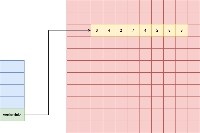
Let’s review how a vector is arranged in memory to understand the layout of our vector of vectors. Remember that a vector stored on the stack makes a heap allocation to store its data, which means that under the hood a vector is using a pointer to keep track of the location of the actual data. Below is an example of a vector of ints (green) stored on the stack (blue), with an allocation (yellow) on the heap (red).
When we have a vector of vectors, each element of the vector’s data is itself a vector, which is pointing to a separate location in memory to store its own data. Below is a diagram of a $5 \times 4$ matrix (5 rows, 4 columns); the vector of vectors point to an allocation on the heap containing 5 vectors (one for each row), which themselves each points to a block of memory 4 ints wide. These blocks of memory can in principle be placed anywhere in memory.
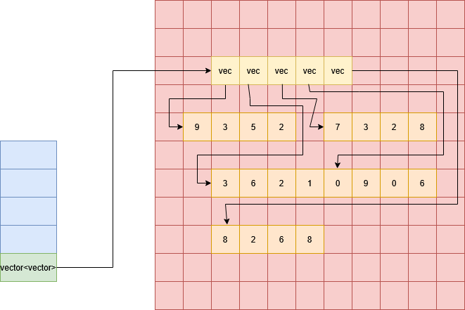
Each row is clearly contigous but the columns are not. For example, the first column of this matrix would be made up of the first element of each row, which are placed independently throughout memory.
The result of using a C-style 2D array (int** Matrix) is the same in terms of memory layout, since a C-style 2D arrays is likewise an array of pointers to arrays.
Multi-Dimesional Arrays in a Contiguous Block
Instead of having all our rows (or columns) placed in independent locations in memory, we can also allocate a contiguous $N \times M$ block of memory to store all of the data that we need, like this:
std::vector<int> Matrix(N*M, 0);
where again we have initialised the matrix to all zeroes.
This represents a matrix as a single “flat” array, so its memory layout is just the same as a regular 1D array. You will find that this is the more common approach in performant applications; this layout reduces memory fragmentation, makes it easier to transfer matrix data as a single contiguous buffer, and allows us to get improved cache performance out of algorithms that iterate over all elements.
The matrix must now be stored in one contiguous block, either row by row (row-major) or column by column (column major). The trick to using this kind of structure is to convert between 2D indices $(i,j)$ (where $0 \le i \lt N$ and $0 \le j \lt M$) to a single index $k$ (where $0 \le k \lt N\times M$). N.B. here we will use the matrix convention where indices $(i,j)$ refer to row $i$ and column $j$.
To understand how to do this, let’s consider a row-major matrix. To find the element $(i,j)$, we are trying to find element $j$ of row $i$; this means that the we just need to find the start of row $i$ and then add $j$. Since the matrix is row-major, the start of row $i$ is at index $M \times i$ (the number of rows before it times the length of a row, which is the number of columns). Therefore our formula for row major indices is:
$k_\text{row-major} = M \times i + j$,
and likewise for indices in column major matrices:
$k_\text{col-major} = N \times j + i$.
Linked Lists
A linked list is a representation of a list that is stored like a graph: each element of the list consists of its data and a pointer to the next element of the list. A linked list has no guarantees of being stored contiguously, so the only way to navigate the linked list is to follow the pointers from one node to the next; this is in contrast to random access arrays. A common extension of the linked list is the doubly-linked list, which has pointers to the next and previous element in a list.
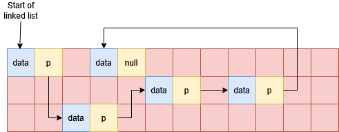
The diagram shows a possible layout linked list nodes in memory. The red grid shows memory locations, blue cells are occupied by a linked list data element and the yellow cells are occupied by a linked list pointer; arrows show the location that each pointer stores. Note the list can be terminated with a null pointer.
Accessing element $i$ of the list requires us to read and follow $i$ pointers, and the amount of work done to find elements increases linearly as the we get further into the list. The advantage of a linked list however is that we can add or remove elements more straightforwardly by simply modifying the relevant pointers. This is much simpler than removing or inserting elements in the middle of a random access array, which requires copying memory to keep all the elements correctly in order.
Linked lists also provide natural representations for various scenarios:
- Singly linked lists can have multiple lists share the same tail.
- Infinite cycles can be easily represented as linked lists without additional book-keeping.
- Linked lists are recursive data structures, which make some algorithms natural to express as simple recursive functions.
std::list is usually implemented as a doubly-linked list, and std::forward_list is usually implemented as a singly-linked list.
Binary Search Trees
A binary search tree (BST) is another graph based structure, where each node consists of its data, and pointers to a left and right sub-tree (the “left child” and “right child”). The data stored in a BST must admit a comparison operator $<$, so that for a given node with data $d$:
- for all data $d_L$ in the left sub-tree, $d_L < d$, and
- for all data $d_R$ in the right sub-tree, $d_R >= d$.
A BST is therefore always sorted w.r.t. keys. It is often used to implement associative arrays, which is a set of key-value pairs that allow look-up of values based on key. You may be familiar with this concept as a dictionary in Python. If the data in a BST is a key-value pair $(k,v)$, then the ordering is just on the key $k$. Looking up a value based on a key requires traversing the tree from its root and comparing the keys to determine whether to look up the left or right sub-tree at each node.
The diagram below shows a BST; the first piece of data (in the blue cell) is the key, followed by value, the left child pointer, and the right child pointer. A null pointer can be used to represent a lack of left or right child. Note that the tree is sorted by the key and is not sorted on values.
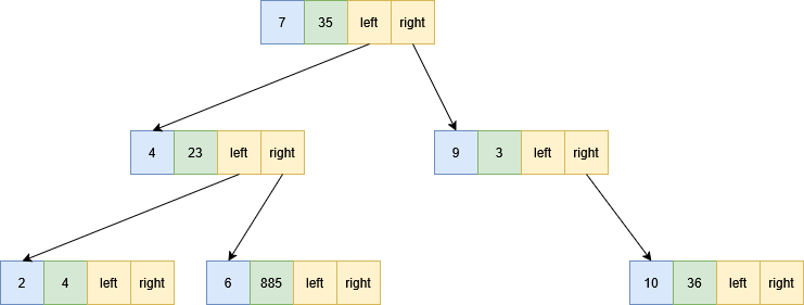
The complexity of many operations on BSTs is determined by the height of the tree. The height of a tree (or subtree) is the maximum length of path that we can take from the top node until we reach a node with no children and can go no further. The diagram above shows a tree of height 3; the subtree starting at the node with $k=4$ has height 2.
Like a linked list, a BST is not necessarily contiguous, and different nodes may be located anywhere in memory. In order to explore a BST for look-up or insertion we have to follow a chain of pointers to find the memory locations of the nodes.
There are variations on BSTs, such as red-black trees, called balanced BSTs. A balanced BST guarantees that the left and right sub-trees of any given node are similar in size. (More precisely, that the height of the left and right sub-tree differ by no more than 1.) These structures avoid the worst case scenarios that we will discuss in class!
std::map is usually implemented as a balanced BST.
Hash Tables
A hash table is an alternative implementation for an associative array. It consists of a “table” in the form of a random access array. In order to find at which index $i$ of the table a key-value pair $(k,v)$ is stored, we have function $i = h(k)$. An ideal hash function is constant time on all keys and minimises the chance of collisions. A collision between two keys $k_1$ and $k_2$ is when $h(k_1) = h(k_2)$. Note that it is not possible for $h$ to be completely collisionless unless you have at least as many rows in your hash table as elements you want to insert. Generally the table stores some kind of list at each index in order to resolve collisions, so in practice you will typically have a random access array of pointers, and each pointer will point to an array (or list, or similar structure) containing all the key-value pairs which hash to that index.
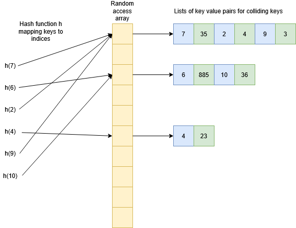
The diagram below gives an example of a hash table for the same data as the BST above. In the ideal case all the keys would map to different indices in the table, but for illustration purposes we have shown a number of collisions. From each hash function on the left we get an index in the random access array, and then we can follow a pointer to all the data stored at that index.
How quick it is to look up an element in this list will depend on the kind of structure used (for example, all of the above structures could be used!) but the key to a hash table’s performance is that collisions should be rare so that the size of these lists remains small. If the number of colliding keys is bounded by a constant then the look-up/insertion in the list will constant time, and since the hash function and checking the random access array are also constant time, hash tables have $O(1)$ operations for insertion, look-up, and removal. Just because the complexity is $O(1)$ (under appropriate circumstances) doesn’t necessarily mean that hash tables are faster than other methods though: there are overheads to think about as well, especially from the hash function! Often a BST will be faster for moderately sized data. Hash tables can also require allocating more memory than you need.
std::unordered_map is usually implemented as a hash table.
Cache Performance of Data-Structures
As we’ve seen from the above, structures like linked lists, binary search trees, and hash tables can be highly fragmented in memory (i.e. they are not necessarily contiguous). This prevents us from getting substantial performance advantage from hardware caching the way that we do when iterating over contiguous arrays. When we can, it is desirable to store data in a so-called “flat” datastructure, i.e. a contiguous block of memory with data stored in an appropriate order. This makes iterating over data faster due to the cache benefits, and also makes data easier to send to external devices such as GPUs or other CPUs (as we’ll see when we explore MPI in weeks 9 and 10).
This does not mean that we shouldn’t use data structures like linked lists or BSTs, but its important to understand the advantages and disadvantages to make informed choices. For example, if we need an associative array of key-value pairs, simply storing them in a random access array would make it very hard to look up the value for a given key. Having a structure like a BST makes this look up fast even though the data is more fragmented.